
- SAP Community
- Products and Technology
- Technology
- Technology Blogs by SAP
- A Multivariate Time Series Modeling and Forecastin...
Technology Blogs by SAP
Learn how to extend and personalize SAP applications. Follow the SAP technology blog for insights into SAP BTP, ABAP, SAP Analytics Cloud, SAP HANA, and more.
Turn on suggestions
Auto-suggest helps you quickly narrow down your search results by suggesting possible matches as you type.
Showing results for
Product and Topic Expert
Options
- Subscribe to RSS Feed
- Mark as New
- Mark as Read
- Bookmark
- Subscribe
- Printer Friendly Page
- Report Inappropriate Content
05-06-2021
3:04 PM
Picture this – you are the manager of a supermarket and would like to forecast the sales in the next few weeks and have been provided with the historical daily sales data of hundreds of products. What kind of problem would you classify this as? Of course, time series modeling, such as ARIMA and exponential smoothing, may come out into your mind naturally. With these tools, you could take sales of each product as separate time series and predict its future sales based on its historical values.
After a minute, you realize that the sales of these products are not independent and there is a certain dependency amongst them. For example, during festivals, the promotion of barbecue meat will also boost the sales of ketchup and other spices. If one brand of toothpaste is on sale, the demand of other brands might decline. Such examples are countless. When there are multiple variables at play, we need to find a suitable tool to deal with such Multivariable Time Series (MTS), which could handle the dependency between variables.
In SAP HANA Predictive Analysis Library(PAL), and wrapped up in the Python Machine Learning Client for SAP HANA(hana-ml), we provide you with one of the most commonly used and powerful methods for MTS forecasting - VectorARIMA which includes a series of algorithms - VAR, VARX, VMA, VARMA, VARMAX, sVARMAX, sVARMAX.
In this blog post, you will learn:
- Introduction of MTS and VectorARIMA.
- A use case containing the steps for VectorARIMA implementation to solidify you understanding of algorithm.
This blog post assumes that you already have some familiarity with univariate time series and ARIMA modeling (AR, MA, ARIMAX, sARIMA, …). In hana-ml, we also provide these tools - ARIMA and AutoARIMA and you could refer to the documentation for further information.
1. Introduction of MTS and VectorARIMA
A Multivariate Time Series consist of more than one time-dependent variable and each variable depends not only on its past values but also has some dependency on other variables.
To deal with MTS, one of the most popular methods is Vector Auto Regressive Moving Average models (VARMA) that is a vector form of autoregressive integrated moving average (ARIMA) that can be used to examine the relationships among several variables in multivariate time series analysis.
In hana-ml, the function of VARMA is called VectorARIMA which supports a series of models, e.g. pure VAR, pure VMA, VARX(VAR with exogenous variables), sVARMA (seasonal VARMA), VARMAX. Similar to ARIMA, building a VectorARIMA also need to select the propriate order of Auto Regressive(AR) p, order of Moving Average(MA) q, degree of differencing d. If the seasonality exists in the time series, seasonal related parameters are also needs to be decided, i.e. seasonal period s, Order of vector seasonal AR P, order of vector seasonal MA Q, Degree of seasonal differencing D.
In VectorARIMA, the orders of VAR/VMA/VARMA models could be specified automatically. Note that the degree of differencing needs to provided by the user and could be achieved by making all time series to be stationary.
In the auto selection of p and q, there are two search options for VARMA model: performing grid search to minimize some information criteria (also applied for seasonal data), or computing the p-value table of the extended cross-correlation matrices (eccm) and comparing its elements with the type I error. VAR model uses grid search to specify orders while VMA model performs multivariate Ljung-Box tests to specify orders.
2. Solutions
In this section, a use case containing the steps for VectorARIMA implementation is shown to solidify you understanding of algorithm.
2.1 Dataset
A public dataset in Yash P Mehra’s 1994 article: “Wage Growth and the Inflation Process: An Empirical Approach” is used and all data is quarterly and covers the period 1959Q1 to 1988Q4. The dataset has 123 rows and 8 columns and the definition of columns are shown below.
- rgnp : Real GNP.
- pgnp : Potential real GNP.
- ulc : Unit labor cost.
- gdfco : Fixed weight deflator for personal consumption expenditure excluding food and energy.
- gdf : Fixed weight GNP deflator.
- gdfim : Fixed weight import deflator.
- gdfcf : Fixed weight deflator for food in personal consumption expenditure.
- gdfce : Fixed weight deflator for energy in personal consumption expenditure.
The download link of dataset.
Visualize the data in the figure below and through our observation, all 8 variables has no obvious seasonality and each curve slopes upward. Hence, in the following analysis, we will not consider the seasonality in the modeling.

Fig. 1. Curves of 8 variables
Source code will use Python machine learning client for SAP HANA Predictive Analsysi Library(PAL).
2.2 SAP HANA Connection
We firstly need to create a connection to a SAP HANA and then we could use various functions of hana-ml to do the data analysis. The following script is an example:
import hana_ml
from hana_ml import dataframe
conn = dataframe.ConnectionContext('host', 'port', 'username', 'password')
2.3 Data Splitting
The dataset has been imported into SAP HANA and the table name is “GNP_DATA”. Hence, we could access to the table via dataframe.ConnectionContext.table() function. Then, we add a column called ‘ID’ to the original DataFrame df as VectorARIMA() requires an integer column as key column. Then, select top 80% of df (i.e. 99 rows) as training data and the rest (i.e. 24 rows) as test data for modeling in the next step.
# The 'date' column in the original csv file has been dropped
df = conn.table('GNP_DATA')
# Add a ID column
df = df.add_id('ID')
# select 80% of data as the training data and the rest as the test data
df_train = df.filter('ID <= 99')
df_test = df.filter('ID > 99')
print(df_train.head(5).collect())
print(df_test.head(5).collect()) 
2.4 Model Building
The data is ready, let's start the trip of MTS modeling! We will involve the steps below:
- Causality investigation
- Test for stationary
- Model Building
- Test for residuals (errors)
2.4.1 Causality Investigation
First, we use Granger Causality Test to investigate causality of data. Granger causality is a way to investigate the causality between two variables in a time series which actually means if a particular variable comes before another in the time series. In the MTS, we will test the causality of all combinations of pairs of variables.
The Null Hypothesis of the Granger Causality Test is that lagged x-values do not explain the variation in y, so the x does not cause y. We use grangercausalitytests function in the package statsmodels to do the test and the output of the matrix is the minimum p-value when computes the test for all lags up to maxlag. The critical value we use is 5% and if the p-value of a pair of variables is smaller than 0.05, we could say with 95% confidence that a predictor x causes a response y.
The script is below:
from statsmodels.tsa.stattools import grangercausalitytests
variables=data.columns
matrix = pd.DataFrame(np.zeros((len(variables), len(variables))), columns=variables, index=variables)
for col in matrix.columns:
    for row in matrix.index:
        test_result = grangercausalitytests(data[[row, col]], maxlag=20, verbose=False)
        p_values = [round(test_result[i+1][0]['ssr_chi2test'][1],4) for i in range(maxlag)]
        min_p_value = np.min(p_values)
        matrix.loc[row, col] = min_p_value
matrix.columns = [var + '_x' for var in variables]
matrix.index = [var + '_y' for var in variables]
print(matrix)
Output:

From the result above, each column represents a predictor x of each variable and each row represents the response y and the p-value of each pair of variables are shown in the matrix. Take the value 0.0212 in (row 1, column 4) as an example, it refers that gdfco_x is causal to rgnp_y. Whereas, the 0.0 in (row 4, column 1) also refers to gdfco_y is the cause of rgnp_x. As all values are all below 0.05 except the diagonal, we could reject that the null hypothesis and this dataset is a good candidate of VectorARIMA modeling.
2.4.2 Stationary Test
As VectorARIMA requires time series to be stationary, we will use one popular statistical test - Augmented Dickey-Fuller Test (ADF Test) to check the stationary of each variable in the dataset. If the stationarity is not achieved, we need to make the data stationary, such as eliminating the trend and seasonality by differencing and seasonal decomposition.
In the following script, we use adfuller function in the statsmodels package for stationary test of each variables. The Null Hypothesis is that the data has unit root and is not stationary and the significant value is 0.05.
from statsmodels.tsa.stattools import adfuller
def adfuller_test(series, sig=0.05, name=''):
    res = adfuller(series, autolag='AIC')
    p_value = round(res[1], 3)
    if p_value <= sig:
        print(f" {name} : P-Value = {p_value} => Stationary. ")
    else:
        print(f" {name} : P-Value = {p_value} => Non-stationary.")

for name, column in data.iteritems():
    adfuller_test(column, name=column.name)
output:

From the results above, we could see none of these varibles is stationary. Let us use the differencing method to make them stationary.
data_differenced = data.diff().dropna()
for name, column in data_differenced.iteritems():
    adfuller_test(column, name=column.name)
output:

Let us do the second differencing:
data_differenced2 = data_differenced.diff().dropna()
for name, column in data_differenced2.iteritems():
    adfuller_test(column, name=column.name)
Output:

Great! All the time series are now stationary and the degree of differencing is 2 that could be used in the model building in the next step.
2.4.3 Model Building
Let's invoke VectorARIMA() function in hana-ml to build a model of MTS in this section.
Commonly, the most difficult and tricky thing in modeling is how to select the appropriate parameters p and q. Many information criterion could be used to measure the goodness of models with various p and q, e.g. AIC, BIC, FPE and HQIC. However, these metrics may select the different values of p and q as optimal results.
Hence, in our VectorARIMA, we provide two search methods - 'grid_search' and 'eccm' for selecting p and q automatically. The grid_search method is popular which could select the model based on a specific information criterion and in our VectorARIMA, AIC and BIC are offered. Sometimes, obtaining the model based on one information criterion is not reliable as it may not be statistically significant. therefore, 'eccm' search method is used to compute the p-value table of the extended cross-correlation matrices (eccm) and comparing its elements with the type I error. When the p-value of a pair of values(p, q) in the eccm is larger than 0.95, we could say it is a good model. In the following experience, we use these two methods and then compare their results.
As we have obtained the degree of differencing d = 2 in the stationary test in Section 2.4.2, we could set d = 2 in the parameter order. For parameter p and q in the order, let's use the automatic selection mechanism and set them to be -1. We also set max_p and max_q to be 5 as large values of p and q and a complex model is not what we prefer.
When search method 'grid_search' is applied:
from hana_ml.algorithms.pal.tsa.vector_arima import VectorARIMA
vectorArima1 = VectorARIMA(order=(-1, 2, -1), model_type = 'VARMA', search_method='grid_search', output_fitted=True, max_p=5, max_q=5)
vectorArima1.fit(data=df_train)
print(vectorArima1.model_.collect())
print(vectorArima1.fitted_.collect())
print(vectorArima1.model_.collect()['CONTENT_VALUE'][3])
output:

From the result vectorArima1.model_.collect()['CONTENT_VALUE'][3] {"D":0,"P":0,"Q":0,"c":0,"d":2,"k":8,"nT":97,"p":4,"q":0,"s":0}, p = 4 and q =0 are selected as the best model, so VAR model is used. Here, as we do not set the value of information_criterion, AIC is used for choosing the best model.
When 'eccm' search method is used:
from hana_ml.algorithms.pal.tsa.vector_arima import VectorARIMA
vectorArima2 = VectorARIMA(order=(-1, 2, -1), model_type = 'VARMA', search_method='eccm', output_fitted=True, max_p=5, max_q=5)
vectorArima2.fit(data=df_train)
print(vectorArima2.model_.collect())
print(vectorArima2.fitted_.collect())
print(vectorArima2.model_.collect()['CONTENT_VALUE'][3])
output:

The result {"D":0,"P":0,"Q":0,"c":0,"d":2,"k":8,"nT":97,"p":3,"q":0,"s":0} shows that p = 3 and q =0, so VAR model is also used.
From the two results above, a VAR model is selected when the search method is "grid_search" and "eccm" and the only difference is the number of AR term. which one is better? Let's explore these two methods based on content of the eccm which is returned in the vectorArima2.model_.collect()['CONTENT_VALUE'][7].
The result of eccm is shown in a row and we need to reshape it to be a matrix for reading easily.
import numpy as np
eccm = np.array ([0.0,0.0,3.3306690738754696e-16,5.1803006329009804e-13,5.6832968331477218e-09,4.6862518318091517e-06,1.9102017719818676e-06,1.6058652447248356e-05,0.0040421371191952105,0.63114408204875216,0.50264616404650142,0.80460590904044849,0.32681926525938776,0.53654390353455961,0.058575416490683652,0.94851217191236303,0.99992902790224059,0.99974296090269166,0.99567691876089359,0.99855563677448467,0.9980628415032069,0.99885722308643166,0.99999997235835603,0.99999975471170444,0.99993274801553744,0.99999998202569551,0.99999995506853501,0.9999999999905026,0.9999999997954333,0.99999999334482903,0.99999863844821002,0.99999999959788133,0.99999999999999756,0.99999999999994793,0.99999999999999223,0.99999999760020342])
eccm = eccm.reshape(6,6)
eccm = pd.DataFrame(np.asmatrix(eccm))
orders = ['0', '1', '2', '3', '4', '5']
eccm.columns = ['q='+ q for q in orders]
eccm.index = ['p='+ p for p in orders]
print(eccm)
Output:

From the eccm, we could tell when p=3 and p=4, q=0, both p-value is greater than 0.95, so both models are good. Another thing we observe is that when p=2 and q=4, the p-value is 0.999 which seems good. However, this model is likely to lead to overfitting.
Hence, we will choose the model (3, 2, 0) to do the following Durbin-Watson statistic to see whether there is a correlation in the residuals in the fitted results.
The null hypothesis of the Durbin-Watson statistic test is that there is no serial correlation in the residuals. This statistic will always be between 0 and 4. The closer to 0 the statistic, the more evidence for positive serial correlation. The closer to 4, the more evidence for negative serial correlation. When the test statistic equals 2, it indicates there is no serial correlation.
from statsmodels.stats.stattools import durbin_watson
residual1 = vectorArima1.fitted_.select('NAMECOL','RESIDUAL').add_id('ID').dropna()
def DW_test(df, columns):
    for name in columns:
        rs = df.loc[df['NAMECOL'] == name, 'RESIDUAL']
        out = durbin_watson(rs)
        print(f'"{name}": "{out}"')
DW_test(df=residual1.collect(), columns=data.columns)
Output:
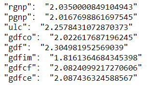
In general, if test statistic is less than 1.5 or greater than 2.5 then there is potentially a serious autocorrelation problem. Otherwise, if test statistic is between 1.5 and 2.5 then autocorrelation is likely not a cause for concern. Hence, the results of residuals in the model (3, 2, 0) look good.
After the implementation above, we will use the model (3, 2, 0) in the next step.
2.5 Model Forecasting
In this section, we will use predict() function of VectorARIMA to get the forecast results and then evaluate the forecasts with df_test. The first return - result_dict1 is the collection of forecasted value. Key is the column name. The second return - result_all1 is the aggerated forecasted values.
result_dict1, result_all1 = vectorArima1.predict(forecast_length=24)
print(result_dict1['rgnp'].head(5).collect())
print(result_all1.head(5).collect())
Ouptut:

Visualize the forecast with actual values:
def plot_forecast_actuals(data, data_actual, data_predict):
    fig, axes = plt.subplots(nrows=int(len(data_actual.columns)/2), ncols=2, dpi=120, figsize=(10,10))
    for i, (col,ax) in enumerate(zip(data.columns, axes.flatten())):
        ax.plot(data_predict[col].select('FORECAST').collect(), label='forecast', marker='o')
        ax.plot(data_actual.collect()[col], label='actual values', marker='x')
        ax.legend(loc='best')
        ax.set_title(data.columns[i])
        ax.set_title(col)
        ax.tick_params(labelsize=6)
    plt.tight_layout();

plot_forecast_actuals(data=data, data_actual=df_test, data_predict=result_dict1)
Output:


Then, use accuracy_measure() function of hana-ml to evaluate the forecasts with metric 'rmse'.
from hana_ml.algorithms.pal.tsa.accuracy_measure import accuracy_measure
def accuracy(pre_data, actual_data, columns):
    for name in columns:
        prediction = pre_data[name].select('IDX', 'FORECAST').rename_columns(['ID_P', 'PREDICTION'])
        actual = actual_data.select(name).add_id('ID').rename_columns(['ID_A', 'ACTUAL'])
        joined = actual.join(prediction, 'ID_P=ID_A').select('ACTUAL', 'PREDICTION')
        am_result = accuracy_measure(data=joined, evaluation_metric=['rmse'])
        rmse = am_result.collect()['STAT_VALUE'][0]
        print(f'"{name}": "{rmse}"')

accuracy(pre_data=result_dict1, actual_data=df_test, columns=data.columns)
Output:

2.6 Impulse Response Function
To explore the relations between variables, VectorARIMA of hana-ml supports the computation of the Impulse Response Function (IRF) of a given VAR or VARMA model. Impulse Response Functions (IRFs) trace the effects of an innovation shock to one variable on the response of all variables in the system.
We could obtain the result of IRF by setting parameter 'calculate_irf' to be True and then the result is returned in an attribute called irf_. An example of VectorARIMA model(3,2,0) is shown below.
vectorArima3 = VectorARIMA(order=(3, 2, 0),
                           model_type = 'VARMA',
                           search_method='eccm',
                           output_fitted=True,
                           max_p=5,
                           max_q=5,
                           calculate_irf=True,
                           irf_lags = 20)
vectorArima3.fit(data=df_train)
print(vectorArima3.irf_.collect().count())
print(vectorArima3.irf_.head(40).collect())
As shown above, vectorArima3.irf_ contains the IRF of 8 variables when all these variables are shocked over the forecast horizon (defined by irf_lags, i.e. IDX column 0 - 19), so the total row number of table is 8*8*20=1280.
From the irf_ table, we could plot 8 figures below and each figure contains 8 line plots representing the responses of a variable when all variables are shocked in the system at time 0. For example, Figure 1 in the top left contains the IRF of the variable 'rgnp' when all variables are shocked at time 0.

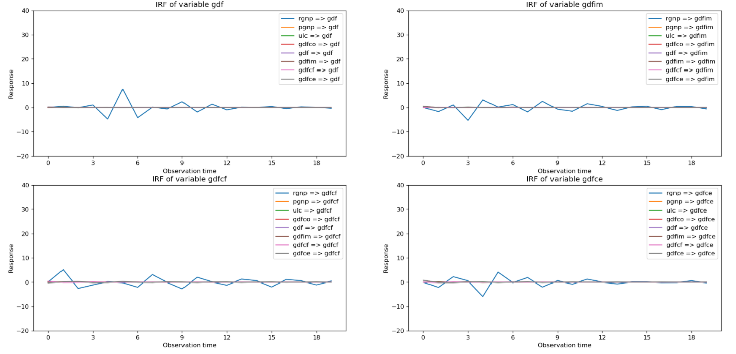
After observation, we can see that the eight figures above have something in common. When the variable 'rgnp' is shocked, the responses of other variables fluctuates greatly. On the contrary, when other variables are shocked, the response of all variables almost does not fluctuate and tends to zero. Hence, the variable 'rgnp' is very important in the system.
3. Summary
In this blog post, we described what is Multi Time Series and some important features of VectorARIMA in hana-ml. We also provide a use case to show the steps of VectorARIMA implementation to solidify you understanding of algorithm. Hope you enjoyed reading this blog post!
If you want to learn more of VectorARIMA function of hana-ml and SAP HANA Predictive Analysis Library (PAL), please refer to the following links:
hana-ml VectorARIMA documentation
SAP HANA Predictive Analysis Library (PAL) VARMA manual
Other Useful Links:
hana-ml on Pypi.
We also provide a R API for SAP HANA PAL called hana.ml.r, please refer to more information on the documentation.
For other blog posts on hana-ml:
- Identification of Seasonality in Time Series with Python Machine Learning Client for SAP HANA
- Outlier Detection using Statistical Tests in Python Machine Learning Client for SAP HANA
- Outlier Detection by Clustering using Python Machine Learning Client for SAP HANA
- Anomaly Detection in Time-Series using Seasonal Decomposition in Python Machine Learning Client for ...
- Outlier Detection with One-class Classification using Python Machine Learning Client for SAP HANA
- Learning from Labeled Anomalies for Efficient Anomaly Detection using Python Machine Learning Client...
- Python Machine Learning Client for SAP HANA
- Import multiple excel files into a single SAP HANA table
- COPD study, explanation and interpretability with Python machine learning client for SAP HANA
- Model Storage with Python Machine Learning Client for SAP HANA
- SAP Managed Tags:
- Machine Learning,
- SAP HANA Cloud,
- Python,
- SQL,
- SAP HANA,
- Big Data
Labels:
You must be a registered user to add a comment. If you've already registered, sign in. Otherwise, register and sign in.
Labels in this area
-
ABAP CDS Views - CDC (Change Data Capture)
2 -
AI
1 -
Analyze Workload Data
1 -
BTP
1 -
Business and IT Integration
2 -
Business application stu
1 -
Business Technology Platform
1 -
Business Trends
1,658 -
Business Trends
105 -
CAP
1 -
cf
1 -
Cloud Foundry
1 -
Confluent
1 -
Customer COE Basics and Fundamentals
1 -
Customer COE Latest and Greatest
3 -
Customer Data Browser app
1 -
Data Analysis Tool
1 -
data migration
1 -
data transfer
1 -
Datasphere
2 -
Event Information
1,400 -
Event Information
70 -
Expert
1 -
Expert Insights
177 -
Expert Insights
336 -
General
1 -
Google cloud
1 -
Google Next'24
1 -
GraphQL
1 -
Kafka
1 -
Life at SAP
780 -
Life at SAP
14 -
Migrate your Data App
1 -
MTA
1 -
Network Performance Analysis
1 -
NodeJS
1 -
PDF
1 -
POC
1 -
Product Updates
4,575 -
Product Updates
378 -
Replication Flow
1 -
REST API
1 -
RisewithSAP
1 -
SAP BTP
1 -
SAP BTP Cloud Foundry
1 -
SAP Cloud ALM
1 -
SAP Cloud Application Programming Model
1 -
SAP Datasphere
2 -
SAP S4HANA Cloud
1 -
SAP S4HANA Migration Cockpit
1 -
Technology Updates
6,872 -
Technology Updates
468 -
Workload Fluctuations
1
Related Content
- Machine Learning Algorithm Selection in Technology Blogs by Members
- New Machine Learning features in SAP HANA Cloud in Technology Blogs by SAP
- Unleashing AI and Machine Learning in Sales: Advanced Price-Volume Forecasting with SAP Analytics Cl in Technology Blogs by SAP
- Predictive Forecast Disaggregation in Technology Blogs by SAP
- Recap — SAP Data Unleashed 2024 in Technology Blogs by Members
Top kudoed authors
| User | Count |
|---|---|
| 18 | |
| 12 | |
| 10 | |
| 8 | |
| 7 | |
| 6 | |
| 6 | |
| 6 | |
| 6 | |
| 6 |