
- SAP Community
- Products and Technology
- Technology
- Technology Blogs by SAP
- Working with the Standalone SAP HANA Cloud Data La...
Technology Blogs by SAP
Learn how to extend and personalize SAP applications. Follow the SAP technology blog for insights into SAP BTP, ABAP, SAP Analytics Cloud, SAP HANA, and more.
Turn on suggestions
Auto-suggest helps you quickly narrow down your search results by suggesting possible matches as you type.
Showing results for
Advisor
Options
- Subscribe to RSS Feed
- Mark as New
- Mark as Read
- Bookmark
- Subscribe
- Printer Friendly Page
- Report Inappropriate Content
07-13-2023
9:29 AM
The previous blog post on “Working with the Embedded Data Lake in SAP Datasphere” outlined how you can realize a cold-to-hot data tiering scenario with SAP Datasphere and the embedded SAP HANA Cloud data lake. As SAP Datasphere also provides the option to easily connect to the standalone SAP HANA Cloud data lake, this blog will show you, how you can read data from the standalone data lake and persist part of that data in-memory to realize the cold-to-hot scenario.
The figure below shows the overall approach for this scenario. First, a connection in SAP Datasphere to the standalone SAP HANA Cloud data lake will be created to be able to read data from the data lake. Once the connection is ready a remote table is created and deployed with which you can access the data from the data lake live without having to replicate the whole data to SAP Datasphere. On top of that four views are created one of which will be snapshotted to demonstrate the cold-to-hot use case. These views will be consumed by SAP Analytics Cloud to measure and compare the performance of query times of cold and hot data.
1. The first thing is to set up the connection to the standalone SAP HANA Cloud data lake. Navigate from the main menu on the left side to the Connections. Choose your space in which you want to set up the connection to the data lake. In this example and to also have the same space names as in the previous blog, the “UK_SPACE” is selected.
2. Next, click on “Create” and search for data lake. Choose the “SAP HANA Cloud, Data Lake Relational Engine.
4. Enter a business name, e.g. “HANA_STANDALONE_DATA_LAKE” & click on “Create Connection”. Once created, you can always click on "Validate" to test if the connection is working fine. This will also give you information about whether Data Flows are enabled and remote tables are supported for this connection.
Now that the connection is successfully established you can start reading data from the data lake. To avoid duplicate data in SAP Datasphere and the source system, data can be accessed live with the help of remote tables. When the remote table is deployed the data stays in the source system and is not replicated to SAP Datasphere. On top of the remote table you can then build graphical or SQL views.
5. Switch to the Data Builder and click on the import icon and select "Import Remote Tables".
6. Next select the connection to the data lake and click “Next Step”. Now select the table you like to import. Choose “Next Step”.
7. You get an overview of the objects that you will import. If an object has already been imported, it is listed on the tab Already in the Repository and will not be imported again. For the objects to be imported, you can change the technical name and the business name.
8. Choose “Import and Deploy”. The import status is displayed. Click on “Close” to close the wizard.
9. In the next steps, similar to the previous blog post on the embedded data lake, 4 graphical views will be created. The first one is a snapshotted view of 2021 data containing about 50 million rows of data. Select the remote table as a source and filter on 2021 data. In the properties set ‘Analytical Dataset’ as a semantic usage, toggle the switch ‘Expose for Consumption’ and set Sales Unit as a measure. Save and deploy the view and name it 2_UK_SALES_2021. When the view is deployed scroll down in the properties panel to the persistency area and create a snapshot. The details of the snapshot you can review in the Data Integration Monitor (View Persistency Monitor).
10. The second view is a non-persisted view for year 2020. Follow the same steps as before, except that no snapshot is created. The name of the view is set to 2_UK_SALES_2020.
11. Thirdly, create a view to combine the 2021 snapshotted data and the 2020 virtual data, which we created in steps 9 & 10. The union can be created by dragging the second view on top of the first view and choosing the union option. Set the same properties as in the previously created views. A snapshot is not created. The name of the view is set to 3_UK_SALES_2020_2021.
12. Lastly, you can also create a view to get 2020 and 2021 data from the data lake directly and compare the query times to the 3_UK_SALES_2020_2021 view. Create a view and filter on the year 2020 and 2021.
13. Next a story in SAP Analytics Cloud is created which loads the data from SAP Datasphere via a live connection and displays it on the canvas. If you have not yet created a live connection please refer to this document.
Create a new Canvas Page and click on Add data. Now choose SAP Datasphere as the data source. Select the connection and choose the respective UK_SPACE. First, select the 2020 Sales data. Add a chart to display the 2020 data.
Next add the 2021 Sales data similar to the previous step and set the charts data source to 2021. Select the measure Sales_Unit again so that the chart displays data. Notice that the data is loaded much faster than before because this view has been persisted in SAP Datasphere and resides in memory unlike 2020 data, which is stored in the data lake.
You can also test the query times for the union view which combines data from the data lake with snapshotted data. Compared to the view were all data resides in the data lake this is about 1.4 times faster. The figure below displays how the data flows through SAP Datasphere to SAP Analytics Cloud and shows the query time differences.
To conclude, this blog has shown how to carry out a Cold-To-Hot data tiering scenario in SAP Datasphere and the standalone SAP HANA Cloud data lake. It showed you how to create a connection to the data lake and consume data in SAP Datasphere live with a remote table. Also, several views were built on top of the remote table, one of which was snapshotted and stored as hot data. The views were then consumed by SAP Analytics Cloud to measure the query times. It made evident, that the access on hot data is much faster and also a hybrid scenario with cold and hot data can improve the performance.
Thank you for reading!
Feel free to also check out this blog about the data architecture with SAP. To learn more about the prerequisites and configuration steps needed to set up a connection take a look at the help documents SAP HANA Cloud, Data Lake Relational Engine and SAP HANA Cloud, Data Lake Files which will provide you the necessary information.
The figure below shows the overall approach for this scenario. First, a connection in SAP Datasphere to the standalone SAP HANA Cloud data lake will be created to be able to read data from the data lake. Once the connection is ready a remote table is created and deployed with which you can access the data from the data lake live without having to replicate the whole data to SAP Datasphere. On top of that four views are created one of which will be snapshotted to demonstrate the cold-to-hot use case. These views will be consumed by SAP Analytics Cloud to measure and compare the performance of query times of cold and hot data.
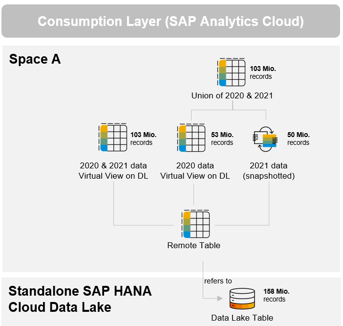
Fig. 1: Architecture Overview
With the following steps, you can realize the cold-to-hot scenario for the standalone SAP HANA Cloud data lake:
1. The first thing is to set up the connection to the standalone SAP HANA Cloud data lake. Navigate from the main menu on the left side to the Connections. Choose your space in which you want to set up the connection to the data lake. In this example and to also have the same space names as in the previous blog, the “UK_SPACE” is selected.
2. Next, click on “Create” and search for data lake. Choose the “SAP HANA Cloud, Data Lake Relational Engine.

Fig. 2: Create a connection
3. Enter the host, port, user name and password and click on “Next Step”.
Fig. 3: Connection properties
4. Enter a business name, e.g. “HANA_STANDALONE_DATA_LAKE” & click on “Create Connection”. Once created, you can always click on "Validate" to test if the connection is working fine. This will also give you information about whether Data Flows are enabled and remote tables are supported for this connection.
Now that the connection is successfully established you can start reading data from the data lake. To avoid duplicate data in SAP Datasphere and the source system, data can be accessed live with the help of remote tables. When the remote table is deployed the data stays in the source system and is not replicated to SAP Datasphere. On top of the remote table you can then build graphical or SQL views.
5. Switch to the Data Builder and click on the import icon and select "Import Remote Tables".
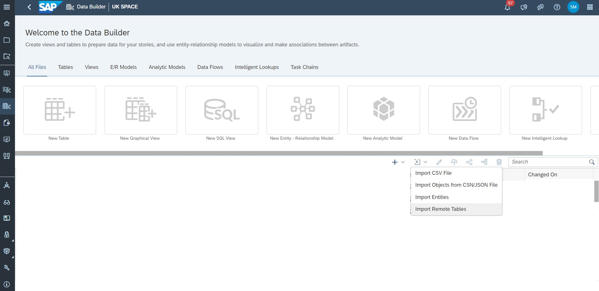
Fig. 4: Import a remote table
6. Next select the connection to the data lake and click “Next Step”. Now select the table you like to import. Choose “Next Step”.
7. You get an overview of the objects that you will import. If an object has already been imported, it is listed on the tab Already in the Repository and will not be imported again. For the objects to be imported, you can change the technical name and the business name.
8. Choose “Import and Deploy”. The import status is displayed. Click on “Close” to close the wizard.
9. In the next steps, similar to the previous blog post on the embedded data lake, 4 graphical views will be created. The first one is a snapshotted view of 2021 data containing about 50 million rows of data. Select the remote table as a source and filter on 2021 data. In the properties set ‘Analytical Dataset’ as a semantic usage, toggle the switch ‘Expose for Consumption’ and set Sales Unit as a measure. Save and deploy the view and name it 2_UK_SALES_2021. When the view is deployed scroll down in the properties panel to the persistency area and create a snapshot. The details of the snapshot you can review in the Data Integration Monitor (View Persistency Monitor).

Fig. 5: Snapshotted graphical view
10. The second view is a non-persisted view for year 2020. Follow the same steps as before, except that no snapshot is created. The name of the view is set to 2_UK_SALES_2020.
11. Thirdly, create a view to combine the 2021 snapshotted data and the 2020 virtual data, which we created in steps 9 & 10. The union can be created by dragging the second view on top of the first view and choosing the union option. Set the same properties as in the previously created views. A snapshot is not created. The name of the view is set to 3_UK_SALES_2020_2021.
12. Lastly, you can also create a view to get 2020 and 2021 data from the data lake directly and compare the query times to the 3_UK_SALES_2020_2021 view. Create a view and filter on the year 2020 and 2021.
13. Next a story in SAP Analytics Cloud is created which loads the data from SAP Datasphere via a live connection and displays it on the canvas. If you have not yet created a live connection please refer to this document.
Create a new Canvas Page and click on Add data. Now choose SAP Datasphere as the data source. Select the connection and choose the respective UK_SPACE. First, select the 2020 Sales data. Add a chart to display the 2020 data.
Next add the 2021 Sales data similar to the previous step and set the charts data source to 2021. Select the measure Sales_Unit again so that the chart displays data. Notice that the data is loaded much faster than before because this view has been persisted in SAP Datasphere and resides in memory unlike 2020 data, which is stored in the data lake.
You can also test the query times for the union view which combines data from the data lake with snapshotted data. Compared to the view were all data resides in the data lake this is about 1.4 times faster. The figure below displays how the data flows through SAP Datasphere to SAP Analytics Cloud and shows the query time differences.

Fig. 6: Overview of Cold vs. Hot Access and Combined Access scenario
Summary
To conclude, this blog has shown how to carry out a Cold-To-Hot data tiering scenario in SAP Datasphere and the standalone SAP HANA Cloud data lake. It showed you how to create a connection to the data lake and consume data in SAP Datasphere live with a remote table. Also, several views were built on top of the remote table, one of which was snapshotted and stored as hot data. The views were then consumed by SAP Analytics Cloud to measure the query times. It made evident, that the access on hot data is much faster and also a hybrid scenario with cold and hot data can improve the performance.
Thank you for reading!
Feel free to also check out this blog about the data architecture with SAP. To learn more about the prerequisites and configuration steps needed to set up a connection take a look at the help documents SAP HANA Cloud, Data Lake Relational Engine and SAP HANA Cloud, Data Lake Files which will provide you the necessary information.
- SAP Managed Tags:
- SAP Datasphere
Labels:
4 Comments
You must be a registered user to add a comment. If you've already registered, sign in. Otherwise, register and sign in.
Labels in this area
-
ABAP CDS Views - CDC (Change Data Capture)
2 -
AI
1 -
Analyze Workload Data
1 -
BTP
1 -
Business and IT Integration
2 -
Business application stu
1 -
Business Technology Platform
1 -
Business Trends
1,658 -
Business Trends
106 -
CAP
1 -
cf
1 -
Cloud Foundry
1 -
Confluent
1 -
Customer COE Basics and Fundamentals
1 -
Customer COE Latest and Greatest
3 -
Customer Data Browser app
1 -
Data Analysis Tool
1 -
data migration
1 -
data transfer
1 -
Datasphere
2 -
Event Information
1,400 -
Event Information
70 -
Expert
1 -
Expert Insights
177 -
Expert Insights
339 -
General
1 -
Google cloud
1 -
Google Next'24
1 -
GraphQL
1 -
Kafka
1 -
Life at SAP
780 -
Life at SAP
14 -
Migrate your Data App
1 -
MTA
1 -
Network Performance Analysis
1 -
NodeJS
1 -
PDF
1 -
POC
1 -
Product Updates
4,575 -
Product Updates
382 -
Replication Flow
1 -
REST API
1 -
RisewithSAP
1 -
SAP BTP
1 -
SAP BTP Cloud Foundry
1 -
SAP Cloud ALM
1 -
SAP Cloud Application Programming Model
1 -
SAP Datasphere
2 -
SAP S4HANA Cloud
1 -
SAP S4HANA Migration Cockpit
1 -
Technology Updates
6,872 -
Technology Updates
470 -
Workload Fluctuations
1
Related Content
- SAC Analytic Application: Table calculation in Technology Q&A
- Tracking HANA Machine Learning experiments with MLflow: A technical Deep Dive in Technology Blogs by SAP
- SAC Story : Recent n Dates calculation in Technology Q&A
- SAP BTP FAQs - Part 1 (General Topics in SAP BTP) in Technology Blogs by SAP
- SAP Datasphere News in April in Technology Blogs by SAP
Top kudoed authors
| User | Count |
|---|---|
| 17 | |
| 12 | |
| 11 | |
| 7 | |
| 7 | |
| 7 | |
| 7 | |
| 6 | |
| 6 | |
| 6 |