
- SAP Community
- Products and Technology
- Technology
- Technology Blogs by SAP
- Working with the Embedded Data Lake in SAP Datasph...
Technology Blogs by SAP
Learn how to extend and personalize SAP applications. Follow the SAP technology blog for insights into SAP BTP, ABAP, SAP Analytics Cloud, SAP HANA, and more.
Turn on suggestions
Auto-suggest helps you quickly narrow down your search results by suggesting possible matches as you type.
Showing results for
Advisor
Options
- Subscribe to RSS Feed
- Mark as New
- Mark as Read
- Bookmark
- Subscribe
- Printer Friendly Page
- Report Inappropriate Content
02-03-2023
7:08 PM
In this blog post you will learn how to realize a Cold-To-Hot data tiering scenario in SAP Datasphere and the embedded SAP HANA Cloud data lake. In this scenario, data will be loaded from a S3 Bucket in AWS into the SAP HANA Cloud data lake using a Data Flow in SAP Datasphere. Part of this data will then be snapshotted and stored as hot in-memory data. The Hot-To-Cold scenario will be covered in a different blog.

Fig. 1: Data Tiering Scenarios
The figure below shows the overall approach for this scenario. First, we will create a new table in the SAP HANA Cloud data lake and a SAP HANA Cloud virtual table which is mapped to that table. The virtual table is used in SAP Datasphere to insert the S3 data into the data lake. Once the data is inserted four views are created one of which contains snapshotted in-memory data. These views will then be consumed by SAP Analytics Cloud to visualize the data and show performance differences in query times. In this example, space names such as “UK_SPACE” are used, however, feel free to set the space names according to your naming convention.

Fig. 2: Architecture Overview
The following steps will guide you through the scenario to set up a Cold-To-Hot data tiering scenario in SAP Datasphere:
1. As a first step, the embedded Data Lake in flexible tenant configuration needs to be configured. Check out more in the following blog.
2. Next, a space needs to be selected that connects to the embedded Data Lake. This can be done in the Space Management in the Overview Tab. Here the checkbox “Use this space to access the data lake” needs to be activated. Note that only one space can be assigned to access the SAP HANA Cloud data lake.

Fig. 3: Space Management
3. A database user needs to be created so that you can access the underlying SAP HANA Cloud database and create the tables. This option can also be found in the Space Management. Create a new database user with read & write privileges and click on “Save”.

Fig. 4: Create a database user
4. Once this is done you can use your preferred SQL tool to create tables in the data lake and access those tables via SAP HANA virtual tables in your open SQL schema. In this blog, the SAP HANA Database Explorer will be used. It can directly be opened from the Space Management via “Open Database Explorer”. In the explorer click on the corresponding instance and enter your credentials to connect to the database.
5. SAP Datasphere offers two stored procedures that you can use to easily create and access the tables. To create tables in the data lake you can use the stored procedure "DWC_GLOBAL"."DATA_LAKE_EXECUTE". Now create a table in the data lake and make sure that the columns’ data types match to the respective S3 data you are going to use.
CALL "DWC_GLOBAL"."DATA_LAKE_EXECUTE"('CREATE TABLE UK_SALES_ACQUISITION (

    Location VARCHAR(40 char),

    Product VARCHAR(40 char),

    Time_ VARCHAR(8 char),

    Sales_Unit DECIMAL(9,1),

    Year VARCHAR(4 char)

)');
Edit 08/07/2023: The create statement was updated with 'char' at the end to ensure that the same semantics (character-length) are used in the SAP HANA Cloud virtual table and the embedded SAP HANA Cloud data lake. For more information, please have a look at the following link.
6. Next you can create a virtual table in your open SQL Schema that refers to the table in the data lake. This can be done with the following procedure:
CALL "DWC_GLOBAL"."DATA_LAKE_CREATE_VIRTUAL_TABLE"

	( VIRTUAL_TABLE_NAME => '0_UK_SALES_ACQUISITION',

      DATA_LAKE_TABLE_NAME => 'UK_SALES_ACQUISITION'

    );
7. Another important step is to grant the space in SAP Datasphere privileges to insert and update the virtual table. Otherwise, the data flow would not be able to insert data into the table. The following procedure will grant the space all privileges:
GRANT ALL PRIVILEGES on "AASPACE_W21_20220921#ONBOARDING"."0_UK_SALES_ACQUISITION"

to AASPACE_W21_20220921 with grant option
8. Now that the virtual table is created, you can go back to SAP Datasphere into your Space with data lake access and create a data flow. To choose the S3 Bucket go to “Sources” -> “Connections” and to your S3 connection. Choose your source file from the S3 bucket and drop it into the canvas of the data flow.
9. The virtual table previously created in the open SQl schema is also available in the sources panel. Drag and drop it onto the canvas of the data flow and click on import and deploy to make it useable as a native SAP Datasphere artefact.

Fig. 5: Add the virtual table to the canvas
Also make sure that it is connected to the source S3 data. A projection node is inserted into the data flow to filter and remove columns that are not needed. In this example, Location, Time, Product and the KPI sales unit are retained. Also, a calculated column Year is created to make it easier to filter on different time periods.

Fig. 6: Create a calculated column
Make sure that the table is set as the target table and all columns are mapped. Also please be aware that currently only APPEND and TRUNCATE modes are supported for the open SQL schema. APPEND with upsert and DELETE are not supported. In the end, the data flow should look like this:

Fig. 7: Data flow to load S3 data into the data lake
10. You can now save and deploy the data flow.
11. Once finished the data flow can be started. Run the data flow and review the status in the Data Integration Monitor. The Data Integration Monitor provides a good overview of all data flow runs. Here you can find information such as last run status, the frequency, duration, start and end timestamps and if set next scheduled runs. In the Record Count you can track how much data has already been transferred to the target.
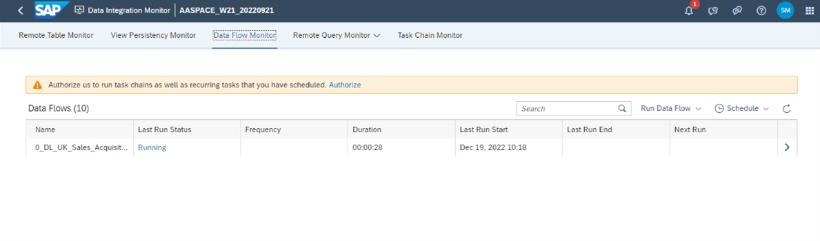
Fig. 8: The Data Flow Monitor
12. After the status of the data flow changed to completed and all the data is transferred into the data lake, share the table into UK_SPACE.
13. The next step is to switch to the UK_SPACE and create a new view based on the shared table. The shared table can be found under Shared Objects. As a first view we want to create a snapshotted view for the Year 2021 which will contain about 50 million rows of data. For this purpose, a filter Year = '2021' is inserted on the Year column. In the properties set ‘Analytical Dataset’ as a semantic usage, toggle the switch ‘Expose for Consumption’ and set Sales Unit as a measure. Save and deploy the View and name it 2_UK_SALES_2021. When the view is deployed scroll down in the properties panel to the persistency area and create a snapshot. The details of the snapshot you can review in the Data Integration Monitor (View Persistency Monitor).
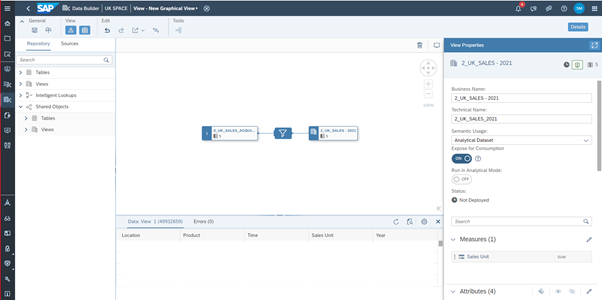
Fig. 9: Data flow to create the table for 2021 sales data

Fig. 10: View Persistency Montor
14. Create View for 2020 Data (non-persisted)
The second view we want to create is a non-persisted view for year 2020 which will contain approx. 53 million rows. To do this, follow the same steps as before, except that no snapshot is created. The name of the view is set to 2_UK_SALES_2020.
15. Create View with Union of 2021 snapshotted and 2020 virtual data
Thirdly, create a view to combine the 2021 snapshotted data and the 2020 virtual data, which we created in steps 13 & 14. The union can be created by dragging the second view on top of the first view and choosing the union option. Set the same properties as in the previously created views. A snapshot is not created. The name of the view is set to 3_UK_SALES_2020_2021.

Fig. 11: Union of two views
16. Create View to combine 2020 and 2021 virtual data
We also want to create a view to get 2020 and 2021 data from the data lake directly and compare the query times to the 3_UK_SALES_2020_2021 view. Create a view and filter on the year 2020 and 2021.
17. Consumption in SAP Analytics Cloud
Next a story in SAP Analytics Cloud is created which loads the data from SAP Datasphere via a live connection and displays it on the canvas. If you have not yet created a live connection please refer to this document.
Create a new Canvas Page and click on Add data. Now choose SAP Datasphere as the data source. Select the connection and choose the respective UK_SPACE. First, select the 2020 Sales data. Add a chart to display the 2020 data.
Next add the 2021 Sales data similar to the previous step and set the charts data source to 2021. Select the measure Sales_Unit again so that the chart displays data. Notice that the data is loaded much faster than before because this view has been persisted in SAP Datasphere and resides in memory unlike 2020 data, which is stored in the data lake.
Edit 07/23: Due to performance improvements the access time for hot data in this example is now even faster with about 60ms.
You can also test the query times for the union view which combines data from the data lake with snapshotted data. Compared to the view were all data resides in the data lake this is about 1.5 times faster. The figure below displays how the data flows through SAP Datasphere to SAP Analytics Cloud and shows the query time differences.

Fig. 12: Overview of Cold vs. Hot Access and Combined Access scenario
Summary
To sum up, this blog has shown how to carry out a Cold-To-Hot data tiering scenario in SAP Datasphere and the embedded SAP HANA Cloud data lake. It was shown that to insert data into the data lake a data lake table and a SAP HANA virtual table in the open SQL schema needs to be created which can then be used in the data flow. After that several views were built on top, one of which was snapshotted and therefore stored as ‘hot’ data. Consuming the views in SAP Analytics Cloud made clear that query times for persisted data were much faster compared to data which resided in the data lake. But of course, it can also be beneficial to store the data in the data lake, e.g. depending on the frequency of data access, volume and how well this data is structured. Especially in times of ever-growing data footprint this provides a great opportunity to better utilize existing resources and optimize your total cost of ownership.
Feel free to also check out this blog which provides valuable insights into SAP Datasphere and the SAP HANA data lake. Also thanks to niga0001, plazi, amoghkulkarni and oliver.herms for their contribution to this blog.
- SAP Managed Tags:
- SAP Datasphere
Labels:
4 Comments
You must be a registered user to add a comment. If you've already registered, sign in. Otherwise, register and sign in.
Labels in this area
-
ABAP CDS Views - CDC (Change Data Capture)
2 -
AI
1 -
Analyze Workload Data
1 -
BTP
1 -
Business and IT Integration
2 -
Business application stu
1 -
Business Technology Platform
1 -
Business Trends
1,661 -
Business Trends
87 -
CAP
1 -
cf
1 -
Cloud Foundry
1 -
Confluent
1 -
Customer COE Basics and Fundamentals
1 -
Customer COE Latest and Greatest
3 -
Customer Data Browser app
1 -
Data Analysis Tool
1 -
data migration
1 -
data transfer
1 -
Datasphere
2 -
Event Information
1,400 -
Event Information
64 -
Expert
1 -
Expert Insights
178 -
Expert Insights
273 -
General
1 -
Google cloud
1 -
Google Next'24
1 -
Kafka
1 -
Life at SAP
784 -
Life at SAP
11 -
Migrate your Data App
1 -
MTA
1 -
Network Performance Analysis
1 -
NodeJS
1 -
PDF
1 -
POC
1 -
Product Updates
4,577 -
Product Updates
326 -
Replication Flow
1 -
RisewithSAP
1 -
SAP BTP
1 -
SAP BTP Cloud Foundry
1 -
SAP Cloud ALM
1 -
SAP Cloud Application Programming Model
1 -
SAP Datasphere
2 -
SAP S4HANA Cloud
1 -
SAP S4HANA Migration Cockpit
1 -
Technology Updates
6,886 -
Technology Updates
403 -
Workload Fluctuations
1
Related Content
- Delete or Clean Error Messages in SAC Story in Technology Q&A
- Datasphere Working Capital Dashboard for SAP S/4HANA content Memory Allocation Error in Technology Q&A
- SAP Cloud Integration: Understanding the XML Digital Signature Standard in Technology Blogs by SAP
- SAP Datapshereでの HANA Cloud, Data Lake の利用方法 in Technology Blogs by SAP
- SAP BTP and Third-Party Cookies Deprecation in Technology Blogs by SAP
Top kudoed authors
| User | Count |
|---|---|
| 12 | |
| 10 | |
| 9 | |
| 7 | |
| 7 | |
| 7 | |
| 6 | |
| 6 | |
| 5 | |
| 4 |