
- SAP Community
- Products and Technology
- Technology
- Technology Blogs by Members
- How to deploy a Natural Language Processing model ...
Technology Blogs by Members
Explore a vibrant mix of technical expertise, industry insights, and tech buzz in member blogs covering SAP products, technology, and events. Get in the mix!
Turn on suggestions
Auto-suggest helps you quickly narrow down your search results by suggesting possible matches as you type.
Showing results for
Former Member
Options
- Subscribe to RSS Feed
- Mark as New
- Mark as Read
- Bookmark
- Subscribe
- Printer Friendly Page
- Report Inappropriate Content
11-30-2020
10:19 AM
Recent advances in Deep learning have led to an astonishing improvement in the methods by which data scientists can create value from large amounts of unstructured text. Nowhere is that more present than in Natural Language Processing (NLP) and in particular, Sentiment Analysis. In this blog post, I will walk you through how you can use TensorFlow’s Python API to construct a simple (relative) deep learning model for sentiment analysis from text and implement it within SAP Data Intelligence. I would like to thank andreas.forster, ffad982802c345bdb6e7377a267f27ce, and karim.mohraz whose blog posts helped give me insight and knowledge that I used to build this blog post. This blog post follows a more recent Text Analysis blog by thorsten.hapke whereby he uses pre-built Deep Learning model along with SpaCy to extract sentiment and Morphological (Named Entity Recognition) information from news articles for visualizations located at, https://blogs.sap.com/2020/10/14/text-analysis-with-sap-data-intelligence/. This blog post will show you , however, how to build the deep learning model for Sentiment Analysis from the ground up in case you have your own data for which you want to train a classifier on.
I will assume that you have:
Now then, let us begin by opening up a Jupyter Notebook in a newly created Scenario in the Machine Learning Scenario Manager interface. We start by importing the necessary libraries:
Then, we shall be using a small dataset in the form of a CSV file that contains 11200 product reviews. However, if you wish, you could use any CSV file so long as it can be imported into Pandas with two columns, text and sentiment/review.
Now, it is always good to perform some exploratory data analysis on the data you get in order to have a good understanding of what you are working with. However, for the purpose of brevity we shall not perform overly too much as I wish to keep this blog post as simple as possible. First, it is good to know what columns you are dealing with as well as the type of hierarchy that the sentiment shall be assessed on:
Index([‘Text’, ‘Ratings’, ‘Cetegories’, ‘Brand’, ‘Manufacturer’, ‘Date’, ‘City’, ‘Province’],
dtype='object')
As one can see, we have an unfortunate distribution of ratings by which those which received a 4 or 5 make up a clear majority. We shall look at stems to mitigate this distribution soon. Now, for our binary classifier, we need to be able to segment these ratings into positive and negative values so we shall convert reviews whose rating goes from 3.0 upwards to a positive class while converting reviews below the threshold to the negative class. The labels for positive and negative reviews will be 1 and 0, respectively.
Next, we shall apply it towards our data and see the distribution afterwards.
Unfortunately, the segmentation has not solved the problem. As such, we are left we 3 choices; first, we can downsample by which we throw out positively labelled reviews until the amount of both classes balance but lose insightful data by doing so, second, we can upsample by which we make copies of the minority class, or we can add weights to the model which penalizes the model heavily for misclassifying the minority class. In this blog post, we shall take the third one so as to retain as much information as possible. Furthermore, we should now begin to preprocess the data. Text typically contain a multitude of non-alpha-numeric characters which would present issues to a machine learning model such as apostrophes or exclamation marks. We shall apply a function that shall remove such characters as well as extra spaces ensuring that only standard text exist.
Now that we have preprocessed the text, it would be a good idea to look at the distribution of words within our corpus. As in, We should see which words are the most common keywords for our data so that we can better understand what we are working on. We shall therefore make a simple graph that can show us these keywords.
As can be inferred from the graph, the dataset is comprised around laptops and the features associated with them such as SSD and screen. Now we shall split the data into train and test sets to be put into the model.
Then, we shall convert the text to a tokenized state using the TensorFlow library’s inbuilt tokenizer. What a tokenizer does is that it converts a sentence to a list of separate words. For example, “I want to go to eat Italian food” would be converted to [‘I’, ‘want’, ‘to’, ‘eat’, ‘Italian’, ‘food’]. This has two purposes; first, it is the necessary format for TensorFlow to accept it as input for models, second, the tokenizer creates an index in the form of a Python dictionary in the background whereby each word now has its own unique number.
If you recall, we had an unfortunate imbalanced dataset where the minority class, negative reviews for this example, was dwarfed by the majority class, positive reviews. If I was to just put in the data into a machine learning model, the model would learn that by just guessing that every review it positive, it could achieve a high accuracy rate, which it would. For that reason, one strategy which shall be implemented would be to give class weights to the model which alter the loss function by assigning more weight to the minority class. This has the effect of increasing the loss incurred if the minority class if mislabeled and therefore ensuring that the model learns to separate both classes. Fortunately, for us, TensorFlow takes this as a single parameter leaving us to only work out how much weight to give to each label.
Now, remember that computers do not understand how to read human language in text form as we do. Because of that, we will convert each review in our text body to numeric form whereby each word is replaced with its unique value in the word index which the tokenizer made for us.
Then, we ‘pad’ the sequences whereby cut off the sentence at a threshold that we decide, hence why it’s useful to look at the word count distribution which we did, and fill up with zeros any sentence whose length is less than the threshold so that all sequences are the same exact length.
Now, we build the deep learning model for our specific task. Please be aware that with deep learning, there is no one size fits all approach. Every single project will require a different model with different parameters fit for its specific task at a specific task. What I am writing here is a generic example that I found works well with the data I have. This may change very easily for any different data.
The last line of code should print out a nice overview of your Deep Learning model so that you can see the change of dimensions within it as well as the number of parameters each layer has. Now we fit the model on the training data and give it the validation data so as to evaluate it. We put it in a variable called history so as to visualize the change in accuracy after.
Running the code will cause the model to train for a predetermined number of epochs on the training data and visualize the predefined metrics per epoch as:
This is great as we see that the model has achieved a final accuracy of about 87% on unseen data. You could of course change the hyper-parameters, run it for longer epochs or get more data to see if you could increase the accuracy. However, for the purpose of keeping this blog as straightforward as possible, I shall leave it up to you to change it to your fancy. We should see our metrics’ progression as the model was going through each epoch. It is always a good idea to check on your metrics progressed throughout the training and we will do so using the following code:
While a confusion matrix may look confusing, no pun intended, it’s quite simple to read it if you see that the bottom right square stands for the amount of positive examples which were correctly labelled as positive whilst the top right square shows how many of the negative examples were classified correctly. As you can see, our model was able to successfully classify both labels extremely well which means that our weights successfully forced it to distinguish between the classes.
Great! We have now built a deep learning model and achieved a good accuracy score of about 87%. Now, we must implement it in pipeline form to have it ready for future inference. If you go on the Machine Learning Scenario Manager interface, scroll down onto the pipeline section and click on the create button and then choose Python Producer Pipeline as the template for a new pipeline, you may name it whatever you wish. By doing so, you will be brought to the modeler page where you will have a pre-built Python consumer graph loaded which will look like:
First, we must specify in the Read File operator which file it is, we wish to train our model on. You must therefore, within the configurations, give the path to the file you want given how you stored it i.e. S3 bucket, HANA database and so forth as such:
In addition to inputting our Python script, the usage of an NLP model requires an additional infrastructure modification. Remember that we had previously created a word index using the TensorFlow tokenizer. This word index is necessary for the model to not only train on data but also to predict future data for inference when deployed. As such, we have to add an additional artifact producer operator to the graph. To do so, first find the artifact producer operator in the operator section on the left. Once you double click on it, it should show up on your screen. Additionally, within the configurations for the Artifact Producer, you must specify a name to be used later for inference. For this blog post, the name shall be wordindex and you should set the Artifact Kind to “Dataset” and the Filename suffix to .CSV as such:
Now, in order to integrate it, we must first right click on the Python operator on the left-hand side and add an output port named wordindex with blob set as its datatype.
Then we can connect the two operators by dragging a connection from the wordindex output port we just made to the “inArtifact” input port for the newly created Artifact Producer. This should look like:
Now, we will add our Python script which will execute the model we created in our Jupyter Notebook instance but within the pipeline. To do so, we must place the equivalent of a Python script version of our notebook, i.e. without visualizations and with api commands to receive and send inputs and outputs from within SAP Data Intelligence. I have already done so for our code and you need to replace the pre-built Python script that is already in the Python operator with this:
In SAP Data Intelligence, you must group your Python Operators with Docker Images so that the required libraries are imported. Right click on the Python Operator and click on group. This should place it within a group for which you will then define the tags that allow SAP Data Intelligence to find the Docker Image you wish to use. For an overview on how to create dockerfiles in case you don't have too much experience with them, please see this tutorial, https://blogs.sap.com/2019/12/13/some-notes-on-docker-file-creation-on-sap-data-intelligence/, by thorsten.hapke.
As of the new 2010 upgrade to SAP Data Intelligence, the Artifact producer Operators must also have a Write File Operator which writes the file into the artifact producer Operator as such. Make sure to connect the output port, “OutFileSend” to the input port for the Write File and then connect the output port of the Write File operator to the input port, “InFile”, for the Artifact Producer Operator.
Now, we must connect the newly created Artifact Producer to the second Python operator which is located on the right-hand side. To do this, we must create a new input port for the second Python operator called wordindex with the datatype of string as such:
Afterwards, we merely drag a connection from the outArtifact port in the Artifact Producer operator to the wordindex input port that we just created. You will be given a small screen which says that you must choose a toString operator to connect them both. Click on the toString operator and you should then see that the two operators are now connected by it as such:
Now, we should change the script within the second Python operator to take this extra connection into account. To do so, replace the script in the second Python operator with this:
This merely checks to make sure that there is output from both artifacts as well as from the metrics operator before it terminated the graph. You should now have a complete graph which looks like:
Now that we have finished building our graph, we can save it and go back the Machine Learning Scenario Manager interface. Go back down towards the pipeline section, click on the pipeline that we have just created and when it’s highlighted, click on execute. The amount of time that this execution will take will depend on how long the model needs to train. This will of course depend on many factors such as the amount of data you have as well as the computational complexity of your model. If you have followed the steps exactly as stated, you should be able to see the Execution completed successfully.
Great, we have now completed the most difficult part of this procedure. We must now build a different pipeline for inference so that we can use the model for new unseen data that we want to classify. Go back to the interface in the machine learning scenario manager and create another pipeline but choose the Python Consumer as the template this time. I’ll name mine Sentiment Inference for simplicity. You will be faced with a screen showing:
Now, just like the training pipeline, we are going to have to modify it slightly to take into account the word index artifact that we had created. TensorFlow will need the word index in order to classify new incoming data. To do this we will have to duplicate the first part of the graph. First, we need to create a new Constant Generator Operator. You can find it in the operator section and then slightly change the content to:
Then, create a toMessage Operator and drag a connection between the newly constant generator to this toMessage Operator via the inString input port. Afterwards, create a new Artifact Consumer operator and drag a connection between the output port of the toMessage Operator and the input port for the Artifact Consumer. Then, we make a toFile operator and connect the outArtifact output port of the Artifact Consumer to the “in” input port of the toFile Operator. The we make a Read File Operator and connect the output of the toFile Operator and the input port of this Read File operator. Furthermore, now we do another similar conversion by making a toBlob Operator and connecting the File Output port of the Read File Operator to the input port to the toBlob Operator. Then Create a new input port in the Python Operator with the blob datatype and call it wordindex. Then, drag a connection between the toBlob Operator’s output port and the Python 3’s new wordindex input port. Hopefully, I haven’t lost you yet with all these conversions. Your graph should now look like:
Now, replace the script within the Python Operator with:
Afterwards, group the Python Operator with the Dockerfile and tags necessary for the relevant packages. Once you have done the following steps, save your graph model and go back to the Machine Learning Scenario Manager interface. Go downwards to the pipelines section, click on your new pipeline and click the deploy button. You will be brought up to a screen asking for configuration description, this is optional, just click on next. You will be brought up to another screen asking if you wish to have previous configurations. Merely press the next button as well and you will be brought to the final step before deployment where it asks you to specify the artifacts to be used in the Inference pipeline. Here, you should click on the drop-down menu and choose the model and word index which were created in the training pipeline.
Once you have done so, click on save. After a bit of processing, your model will be deployed, and you should see a screen of it being run as such:
Now, since we will be using POSTMAN to issue the POST request to have the model classify data we send it via JSON, we will be needing the deployment URL which will be available on the top of the same screen. Copy this and head on over to the POSTMAN interface. At this point, I will have to refer you to andreas.forster’s blog post, https://blogs.sap.com/2019/08/14/sap-data-intelligence-create-your-first-ml-scenario/, on deploying a machine learning model with SAP Data Intelligence online with POSTMAN as he covers exactly what steps you need to do to get POSTMAN working. Once, you have put in the necessary parameters, you merely need to write whatever text you want to have classified and click on send to receive the both the classification (as in positive or negative in binary form) as well as the degree of polarity(a float between 0 and 1 determining the degree to how positive or negative the text is) from the deployed model. Now, as the dataset I used was for the review of laptops and computers, I have written:
{
"text": "I thought the computer was amazing and the processor was so fast!"
}
Unsurprisingly, I receive the degree of sentiment which is .999 indicating it to be extremely positive as it is nearly 1 as well as the classification of 1 meaning it is positive. Please remember that Deep Learning models in general will perform best on data which matches that with which it was trained i.e. a review of a laptop for the data I used may get classified well but a Tweet talking about a new song may achieve poor results. Congratulations, we have now built a basic Natural Language Processing model with TensorFlow for sentiment analysis on SAP Data Intelligence. I have tried to keep things as simple as possible so as to ensure that you know the basic infrastructure to develop NLP models on SAP Data Intelligence. What I have described here can be modified tremendously to fit most tasks involving text and deep learning and it is up to your choice as to what you wish to do with it. Nothing is impossible.
Furthermore, I have written another blogpost detailing what values one could derive from sentiment analysis models such as this one which showcases the practical application of such NLP models here, https://blogs.sap.com/2020/12/22/__trashed-31/.
I will assume that you have:
- A working instance of SAP Data Intelligence
- Basic Python Programming language Skills.
- Customer Review Data (This can be literally any dataset from any datasource such as Kaggle where you have both a column of text reviews and another column of ratings.)
- Please note that Deep Learning works best when there is a lot of data as in thousands of ratings. If you try to build even a basic deep learning model with a small amount of data, you may see sub-optimal results.
Now then, let us begin by opening up a Jupyter Notebook in a newly created Scenario in the Machine Learning Scenario Manager interface. We start by importing the necessary libraries:
import numpy as np

import pandas as pd

import tensorflow as tf

import h5py

import re

from tensorflow.keras.preprocessing.text import Tokenizer

from tensorflow.keras.preprocessing.sequence import pad_sequences

from tensorflow.keras.utils import to_categorical

from tensorflow.keras import Input, Model

from tensorflow.keras.optimizers import Adam

from tensorflow.keras.layers import Flatten, LSTM, Dense, Embedding, Bidirectional

from ipywidgets import IntProgress

from sklearn.model_selection import train_test_split

from sklearn.metrics import confusion_matrix

import seaborn as sns

import matplotlib.pyplot as plt

from sklearn.feature_extraction.text import CountVectorizer

from spacy.lang.en import English

from spacy.lang.en.stop_words import STOP_WORDS

from yellowbrick.text import FreqDistVisualizer

nlp = English()

%matplotlib inline
Then, we shall be using a small dataset in the form of a CSV file that contains 11200 product reviews. However, if you wish, you could use any CSV file so long as it can be imported into Pandas with two columns, text and sentiment/review.
df = pd.read_csv('data/08252020.csv')Now, it is always good to perform some exploratory data analysis on the data you get in order to have a good understanding of what you are working with. However, for the purpose of brevity we shall not perform overly too much as I wish to keep this blog post as simple as possible. First, it is good to know what columns you are dealing with as well as the type of hierarchy that the sentiment shall be assessed on:
df.columnsIndex([‘Text’, ‘Ratings’, ‘Cetegories’, ‘Brand’, ‘Manufacturer’, ‘Date’, ‘City’, ‘Province’],
dtype='object')
sns.countplot(x=df.Ratings)
As one can see, we have an unfortunate distribution of ratings by which those which received a 4 or 5 make up a clear majority. We shall look at stems to mitigate this distribution soon. Now, for our binary classifier, we need to be able to segment these ratings into positive and negative values so we shall convert reviews whose rating goes from 3.0 upwards to a positive class while converting reviews below the threshold to the negative class. The labels for positive and negative reviews will be 1 and 0, respectively.
def to_sentiment(rating):

    rating = int(rating)

    if rating <= 2:

        return 0

    else:

        return 1
Next, we shall apply it towards our data and see the distribution afterwards.
df['Sentiment'] = df['Ratings'].apply(to_sentiment)

class_names = ['negative', 'positive']


ax = sns.countplot(x=df.Sentiment)

plt.xlabel('Review Sentiment')

ax.set_xticklabels(class_names)

Unfortunately, the segmentation has not solved the problem. As such, we are left we 3 choices; first, we can downsample by which we throw out positively labelled reviews until the amount of both classes balance but lose insightful data by doing so, second, we can upsample by which we make copies of the minority class, or we can add weights to the model which penalizes the model heavily for misclassifying the minority class. In this blog post, we shall take the third one so as to retain as much information as possible. Furthermore, we should now begin to preprocess the data. Text typically contain a multitude of non-alpha-numeric characters which would present issues to a machine learning model such as apostrophes or exclamation marks. We shall apply a function that shall remove such characters as well as extra spaces ensuring that only standard text exist.
def preprocess(text):


    # Convert words to lower case and split them

    text = str(text).lower().split()


    # Clean the text

    text = re.sub(r"<br />", " ", str(text))

    text = re.sub(r"[^a-z]", " ", str(text))

    text = re.sub(r"   ", " ", str(text))

    text = re.sub(r"  ", " ", str(text))


    # Return a list of words

    return (text)


def remove_stopwords(text):

    string = nlp(text)

    tokens = []

    clean_text = []

    for word in string:

        tokens.append(word.text)

    for token in tokens:

        idx = nlp.vocab[token]

        if idx.is_stop is False:

            clean_text.append(token)

    return ' '.join(clean_text)


df[‘Text’] = df[‘Text’].apply(preprocess)

df['Text'] = df['Text'].apply(remove_stopwords)
Now that we have preprocessed the text, it would be a good idea to look at the distribution of words within our corpus. As in, We should see which words are the most common keywords for our data so that we can better understand what we are working on. We shall therefore make a simple graph that can show us these keywords.
def word_distribution(text):


    vectorizer = CountVectorizer()

    docs = vectorizer.fit_transform(text)

    features = vectorizer.get_feature_names()


    visualizer = FreqDistVisualizer(features=features, orient='v')

    visualizer.fit(docs)

    visualizer.show()


word_distribution(df['Text'])

As can be inferred from the graph, the dataset is comprised around laptops and the features associated with them such as SSD and screen. Now we shall split the data into train and test sets to be put into the model.
X_train, X_test, y_train, y_test = train_test_split(df['Text'], df['Sentiment'], test _size=0.3)Then, we shall convert the text to a tokenized state using the TensorFlow library’s inbuilt tokenizer. What a tokenizer does is that it converts a sentence to a list of separate words. For example, “I want to go to eat Italian food” would be converted to [‘I’, ‘want’, ‘to’, ‘eat’, ‘Italian’, ‘food’]. This has two purposes; first, it is the necessary format for TensorFlow to accept it as input for models, second, the tokenizer creates an index in the form of a Python dictionary in the background whereby each word now has its own unique number.
tokenizer = Tokenizer()

tokenizer.fit_on_texts(X_train)

word_index = tokenizer.word_index # The word index needs to be used for later

vocab_size = len(word_index) + 1 # We need the vocab size as an argument later

max_len = 250

embedding_dim = 200
If you recall, we had an unfortunate imbalanced dataset where the minority class, negative reviews for this example, was dwarfed by the majority class, positive reviews. If I was to just put in the data into a machine learning model, the model would learn that by just guessing that every review it positive, it could achieve a high accuracy rate, which it would. For that reason, one strategy which shall be implemented would be to give class weights to the model which alter the loss function by assigning more weight to the minority class. This has the effect of increasing the loss incurred if the minority class if mislabeled and therefore ensuring that the model learns to separate both classes. Fortunately, for us, TensorFlow takes this as a single parameter leaving us to only work out how much weight to give to each label.
weight_for_0 = (1 / df['Sentiment'].value_counts()[0])*(len(df))/2.0

weight_for_1 = (1 / df['Sentiment'].value_counts()[1])*(len(df))/2.0


class_weights = {0: weight_for_0, 1: weight_for_1}
Now, remember that computers do not understand how to read human language in text form as we do. Because of that, we will convert each review in our text body to numeric form whereby each word is replaced with its unique value in the word index which the tokenizer made for us.
X_train = tokenizer.texts_to_sequences(X_train)

X_test = tokenizer.texts_to_sequences(X_test)
Then, we ‘pad’ the sequences whereby cut off the sentence at a threshold that we decide, hence why it’s useful to look at the word count distribution which we did, and fill up with zeros any sentence whose length is less than the threshold so that all sequences are the same exact length.
X_train_pad = pad_sequences(X_train, padding='post', maxlen=max_len)

X_test_pad = pad_sequences(X_test, padding='post', maxlen=max_len)
Now, we build the deep learning model for our specific task. Please be aware that with deep learning, there is no one size fits all approach. Every single project will require a different model with different parameters fit for its specific task at a specific task. What I am writing here is a generic example that I found works well with the data I have. This may change very easily for any different data.
inputs = tf.keras.Input(shape=(max_length,))

embedding = tf.keras.layers.Embedding(vocab_size, embedding_dim,


                                      input_length=max_length,

                                      trainable=False)(inputs)

logits = Bidirectional(LSTM(128, dropout=.2, return_sequences=True, recurrent_dropout=.2,

                            kernel_regularizer=tf.keras.regularizers.L2(0.01)))(embedding)

output = Dense(1, activation='sigmoid')(logits)


model = Model(inputs=inputs, outputs=output)

optimizer = Adam(learning_rate=0.001, beta_1=0.9, beta_2=0.995)

model.compile(optimizer=optimizer,

              loss='binary_crossentropy', metrics=['acc'])

model.summary()

The last line of code should print out a nice overview of your Deep Learning model so that you can see the change of dimensions within it as well as the number of parameters each layer has. Now we fit the model on the training data and give it the validation data so as to evaluate it. We put it in a variable called history so as to visualize the change in accuracy after.
history = model.fit(X_train_pad, y_train, batch_size=34, epochs=5, verbose=1,

                    validation_data=(X_test_pad, y_test), class_weight=class_weights)
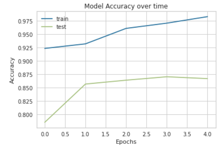
Running the code will cause the model to train for a predetermined number of epochs on the training data and visualize the predefined metrics per epoch as:

This is great as we see that the model has achieved a final accuracy of about 87% on unseen data. You could of course change the hyper-parameters, run it for longer epochs or get more data to see if you could increase the accuracy. However, for the purpose of keeping this blog as straightforward as possible, I shall leave it up to you to change it to your fancy. We should see our metrics’ progression as the model was going through each epoch. It is always a good idea to check on your metrics progressed throughout the training and we will do so using the following code:
plt.plot(history.history['acc'])

plt.plot(history.history['val_acc'])

plt.title('Model Accuracy over time')

plt.ylabel('Accuracy')

plt.xlabel('Epochs')

plt.legend(['train', 'test'], loc='upper left')

plt.show()
While a confusion matrix may look confusing, no pun intended, it’s quite simple to read it if you see that the bottom right square stands for the amount of positive examples which were correctly labelled as positive whilst the top right square shows how many of the negative examples were classified correctly. As you can see, our model was able to successfully classify both labels extremely well which means that our weights successfully forced it to distinguish between the classes.
Great! We have now built a deep learning model and achieved a good accuracy score of about 87%. Now, we must implement it in pipeline form to have it ready for future inference. If you go on the Machine Learning Scenario Manager interface, scroll down onto the pipeline section and click on the create button and then choose Python Producer Pipeline as the template for a new pipeline, you may name it whatever you wish. By doing so, you will be brought to the modeler page where you will have a pre-built Python consumer graph loaded which will look like:

First, we must specify in the Read File operator which file it is, we wish to train our model on. You must therefore, within the configurations, give the path to the file you want given how you stored it i.e. S3 bucket, HANA database and so forth as such:

In addition to inputting our Python script, the usage of an NLP model requires an additional infrastructure modification. Remember that we had previously created a word index using the TensorFlow tokenizer. This word index is necessary for the model to not only train on data but also to predict future data for inference when deployed. As such, we have to add an additional artifact producer operator to the graph. To do so, first find the artifact producer operator in the operator section on the left. Once you double click on it, it should show up on your screen. Additionally, within the configurations for the Artifact Producer, you must specify a name to be used later for inference. For this blog post, the name shall be wordindex and you should set the Artifact Kind to “Dataset” and the Filename suffix to .CSV as such:

Now, in order to integrate it, we must first right click on the Python operator on the left-hand side and add an output port named wordindex with blob set as its datatype.

Then we can connect the two operators by dragging a connection from the wordindex output port we just made to the “inArtifact” input port for the newly created Artifact Producer. This should look like:

Now, we will add our Python script which will execute the model we created in our Jupyter Notebook instance but within the pipeline. To do so, we must place the equivalent of a Python script version of our notebook, i.e. without visualizations and with api commands to receive and send inputs and outputs from within SAP Data Intelligence. I have already done so for our code and you need to replace the pre-built Python script that is already in the Python operator with this:
import numpy as np

import pandas as pd

import tensorflow as tf

import h5py

import re

import logging

import json

import io

import spacy

from tensorflow.keras.preprocessing.text import Tokenizer

from tensorflow.keras.preprocessing.sequence import pad_sequences

from tensorflow.keras.utils import to_categorical

from tensorflow.keras import Input, Model

from tensorflow.keras.optimizers import Adam

from tensorflow.keras.layers import Flatten, LSTM, Dense, Embedding, Bidirectional

from ipywidgets import IntProgress

from sklearn.model_selection import train_test_split

from sklearn.feature_extraction.text import CountVectorizer

from spacy.lang.en import English

from spacy.lang.en.stop_words import STOP_WORDS

nlp = English()


logging.basicConfig(level=logging.DEBUG, format='%(asctime)s - %(levelname)s - %(message)s')


def remove_stopwords(text):

    '''Remove all stopwords such as a, the, and, etc. '''

    string = nlp(text)

    tokens = []

    clean_text = []

    for word in string:

        tokens.append(word.text)

    for token in tokens:

        idx = nlp.vocab[token]

        if idx.is_stop is False:

            clean_text.append(token)

    return ' '.join(clean_text)


def to_sentiment(rating):

    rating = int(rating)

    if rating <= 2:

        return 0

    else:

        return 1


def preprocess(text):

    '''Clean the text, with the option to remove stopwords'''


    # Convert words to lower case and split them

    text = str(text).lower().split()


    # Clean the text

    text = re.sub(r"<br />", " ", str(text))

    text = re.sub(r"[^a-z]", " ", str(text))

    text = re.sub(r"   ", " ", str(text))

    text = re.sub(r"  ", " ", str(text))


    # Return a list of words

    return (text)


def on_input(data):


    api.logger.info("Successfully Started.")

    df = pd.read_csv(io.StringIO(str(data)), engine='python', encoding='utf-8')

    api.logger.info("CSV file imported and read from S3 bucket")

    df = pd.concat([df['reviews.text'], df['reviews.rating']], axis=1, keys=['Text', 'Ratings'])

    api.logger.info('Pandas file successfully completed.')

    # df.dropna(axis=1, inplace=True)


    df['Sentiment'] = df['Ratings'].apply(to_sentiment)

    df['Text'] = df['Text'].apply(preprocess)

    df['Text'] = df['Text'].apply(remove_stopwords)


    X_train, X_test, y_train, y_test = train_test_split(df['Text'],

                                                        df['Sentiment'],

                                                        test_size=0.3)


    X_train = np.array(X_train.values.tolist())

    X_test = np.array(X_test.values.tolist())

    y_train = np.array(y_train.values.tolist())

    y_test = np.array(y_test.values.tolist())


    tokenizer = Tokenizer(oov_token='<OOV>')

    tokenizer.fit_on_texts(X_train)

    api.logger.info('Tokenizer fit onto words!')

    word_index = tokenizer.word_index

    api.logger.info('Index created.')

    vocab_size = len(word_index) + 1


    embedding_dim = 200

    max_length = 250

    pad_type = 'post'


    weight_for_0 = (1 / df['Sentiment'].value_counts()[0])*(len(df))/2.0

    weight_for_1 = (1 / df['Sentiment'].value_counts()[1])*(len(df))/2.0


    class_weights = {0: weight_for_0, 1: weight_for_1}


    X_train = tokenizer.texts_to_sequences(X_train)

    X_test = tokenizer.texts_to_sequences(X_test)

    api.logger.info('texts successfully tokenized')


    X_train_pad = pad_sequences(X_train, padding='post', maxlen=max_length)

    X_test_pad = pad_sequences(X_test, padding='post', maxlen=max_length)


    inputs = tf.keras.Input(shape=(max_length,))

    embedding = tf.keras.layers.Embedding(vocab_size, embedding_dim,

                                          input_length=max_length, mask_zero=True, # The mask is needed to tell the model that the zeros are padding

                                          trainable=False)(inputs)

    logits = Bidirectional(LSTM(128, dropout=.2, return_sequences=False, recurrent_dropout=.2,

                                kernel_regularizer=tf.keras.regularizers.L2(0.01)))(embedding)

    output = Dense(1, activation='sigmoid')(logits)


    model = Model(inputs=inputs, outputs=output)

    optimizer = Adam(learning_rate=0.001, beta_1=0.9, beta_2=0.995)

    model.compile(optimizer=optimizer,

                  loss='binary_crossentropy', metrics=['acc'])

    api.logger.info('Model Successfully built')


    model.fit(X_train_pad, y_train, batch_size=34, epochs=5, verbose=1,

                    validation_data=(X_test_pad, y_test), class_weight=class_weights)

    api.logger.info('Model Successfully Trained')


    loss, acc = model.evaluate(X_test_pad, y_test, steps=34)


    # to send metrics to the Submit Metrics operator, create a Python dictionary of key-value pairs

    metrics_dict = {"loss": str(loss), "accuracy": str(acc)}


    # send the metrics to the output port - Submit Metrics operator will use this to persist the metrics

    api.send("metrics", api.Message(metrics_dict))


    word_index = {y:x for x, y in word_index.items()}

    dict_df = pd.DataFrame.from_dict(word_index, orient='index', columns=['word'])

    api.logger.info(dict_df)

    word_index_file = dict_df.to_csv(index=False)

    api.send('wordindex', word_index_file)


    with h5py.File('trained_model', driver='core', backing_store=False) as model_h5:

        model.save(model_h5)

        model_h5.flush()

        blob = model_h5.id.get_file_image()

        api.send("modelBlob", blob)


api.set_port_callback("input", on_input)
In SAP Data Intelligence, you must group your Python Operators with Docker Images so that the required libraries are imported. Right click on the Python Operator and click on group. This should place it within a group for which you will then define the tags that allow SAP Data Intelligence to find the Docker Image you wish to use. For an overview on how to create dockerfiles in case you don't have too much experience with them, please see this tutorial, https://blogs.sap.com/2019/12/13/some-notes-on-docker-file-creation-on-sap-data-intelligence/, by thorsten.hapke.
As of the new 2010 upgrade to SAP Data Intelligence, the Artifact producer Operators must also have a Write File Operator which writes the file into the artifact producer Operator as such. Make sure to connect the output port, “OutFileSend” to the input port for the Write File and then connect the output port of the Write File operator to the input port, “InFile”, for the Artifact Producer Operator.

Now, we must connect the newly created Artifact Producer to the second Python operator which is located on the right-hand side. To do this, we must create a new input port for the second Python operator called wordindex with the datatype of string as such:

Afterwards, we merely drag a connection from the outArtifact port in the Artifact Producer operator to the wordindex input port that we just created. You will be given a small screen which says that you must choose a toString operator to connect them both. Click on the toString operator and you should then see that the two operators are now connected by it as such:

Now, we should change the script within the second Python operator to take this extra connection into account. To do so, replace the script in the second Python operator with this:
# When both input ports signals arive, the Artifact Producer & Submit Metrics have completed - safe to terminate the graph.


def on_inputs_ready(metrics_resp, artifact_id, wordindex):

    # both input ports have data - previous operators have completed. Send a message as output to stop the graph

    api.send("output", api.Message("Operators complete."))


api.set_port_callback(["metricsResponse", "artifactId", "wordindex"], on_inputs_ready)
This merely checks to make sure that there is output from both artifacts as well as from the metrics operator before it terminated the graph. You should now have a complete graph which looks like:

Now that we have finished building our graph, we can save it and go back the Machine Learning Scenario Manager interface. Go back down towards the pipeline section, click on the pipeline that we have just created and when it’s highlighted, click on execute. The amount of time that this execution will take will depend on how long the model needs to train. This will of course depend on many factors such as the amount of data you have as well as the computational complexity of your model. If you have followed the steps exactly as stated, you should be able to see the Execution completed successfully.

Great, we have now completed the most difficult part of this procedure. We must now build a different pipeline for inference so that we can use the model for new unseen data that we want to classify. Go back to the interface in the machine learning scenario manager and create another pipeline but choose the Python Consumer as the template this time. I’ll name mine Sentiment Inference for simplicity. You will be faced with a screen showing:

Now, just like the training pipeline, we are going to have to modify it slightly to take into account the word index artifact that we had created. TensorFlow will need the word index in order to classify new incoming data. To do this we will have to duplicate the first part of the graph. First, we need to create a new Constant Generator Operator. You can find it in the operator section and then slightly change the content to:

Then, create a toMessage Operator and drag a connection between the newly constant generator to this toMessage Operator via the inString input port. Afterwards, create a new Artifact Consumer operator and drag a connection between the output port of the toMessage Operator and the input port for the Artifact Consumer. Then, we make a toFile operator and connect the outArtifact output port of the Artifact Consumer to the “in” input port of the toFile Operator. The we make a Read File Operator and connect the output of the toFile Operator and the input port of this Read File operator. Furthermore, now we do another similar conversion by making a toBlob Operator and connecting the File Output port of the Read File Operator to the input port to the toBlob Operator. Then Create a new input port in the Python Operator with the blob datatype and call it wordindex. Then, drag a connection between the toBlob Operator’s output port and the Python 3’s new wordindex input port. Hopefully, I haven’t lost you yet with all these conversions. Your graph should now look like:

Now, replace the script within the Python Operator with:
import io

import h5py

import json

import tensorflow as tf

import pandas as pd

from tensorflow.keras.preprocessing.text import Tokenizer

from tensorflow.keras.preprocessing.sequence import pad_sequences

from tensorflow.keras import Model


# Global vars to keep track of model status

model = None

model_ready = False

word_index = None


# Validate input data is JSON

def is_json(data):

  try:

    json_object = json.loads(data)

  except ValueError as e:

    return False

  return True


# When Model Blob reaches the input port

def on_model(model_blob):

    global model

    global model_ready


    model = model_blob

    model_ready = True

    api.logger.info("Model Received & Ready")


def on_word_index(word_index_blob):

    global word_index

    word_index_ = pd.read_csv(io.StringIO(str(word_index_blob,'utf-8')))

    word_index = word_index_.to_dict()['word']

    word_index = {y:x for x, y in word_index.items()}


    api.logger.info(word_index)

    if word_index != None:

        api.logger.info("Word index successfully loaded.")

        api.logger.info(word_index)

    else:

        api.logger.info('Word Index not successfully loaded.')

        api.logger.info(word_index_blob)


# Client POST request received

def on_input(msg):

    global model

    global word_index

    error_message = ""

    success = False

    prediction = None


    def idx_fetch(text, word_index):

        list_ = []

        api.logger.info(word_index)

        for word in text.split():

            api.logger.info(word)

            try:

                list_.append(word_index[word.lower()])

            except:

                list_.append(word_index['<OOV>'])

        return list_


    def get_prediction(model, text, word_index):

        word_list = idx_fetch(text, word_index)

        x = ([word_list])

        sequence = tf.keras.preprocessing.sequence.pad_sequences(x, maxlen=250)

        sentiment = model.predict(sequence)[0]

        if sentiment >= 0.5:

            return (sentiment.item(), 1)

        else:

            return (sentiment.item(), 0)


    try:


        if model_ready:

            api.logger.info("Model Ready")


            user_data = msg.body.decode('utf-8')

            # Received message from client, verify json data is valid

            if is_json(user_data):


                # apply your model

                with io.BytesIO(model) as blob:

                    f = h5py.File(blob, 'r')

                    nnmodel = tf.keras.models.load_model(f)

                    api.logger.info('Model successfully loaded.')


                # obtain your results

                text = json.loads(user_data)["text"]

                api.logger.info('Data successfully partitioned.')

                prediction = get_prediction(nnmodel, text, word_index)

                api.logger.info('Prediction was successful')

                success = True

            else:

                api.logger.info("Invalid JSON received from client - cannot apply model.")

                error_message = "Invalid JSON provided in request: " + user_data

                success = False

        else:

            error_message = "Model has not yet reached the input port - try again."

    except Exception as e:

        error_message = 'An Error occurred: ' + e


    if success:

        # apply carried out successfully, send a response to the user

        msg.body = json.dumps({'Sentiment Prediction': str(prediction)})

    else:

        msg.body = json.dumps({'Error': error_message})


    new_attributes = {'message.request.id': msg.attributes['message.request.id']}

    msg.attributes =  new_attributes

    api.send('output', msg)


api.set_port_callback("model", on_model)

api.set_port_callback("wordindex", on_word_index)

api.set_port_callback("input", on_input)
Afterwards, group the Python Operator with the Dockerfile and tags necessary for the relevant packages. Once you have done the following steps, save your graph model and go back to the Machine Learning Scenario Manager interface. Go downwards to the pipelines section, click on your new pipeline and click the deploy button. You will be brought up to a screen asking for configuration description, this is optional, just click on next. You will be brought up to another screen asking if you wish to have previous configurations. Merely press the next button as well and you will be brought to the final step before deployment where it asks you to specify the artifacts to be used in the Inference pipeline. Here, you should click on the drop-down menu and choose the model and word index which were created in the training pipeline.

Once you have done so, click on save. After a bit of processing, your model will be deployed, and you should see a screen of it being run as such:
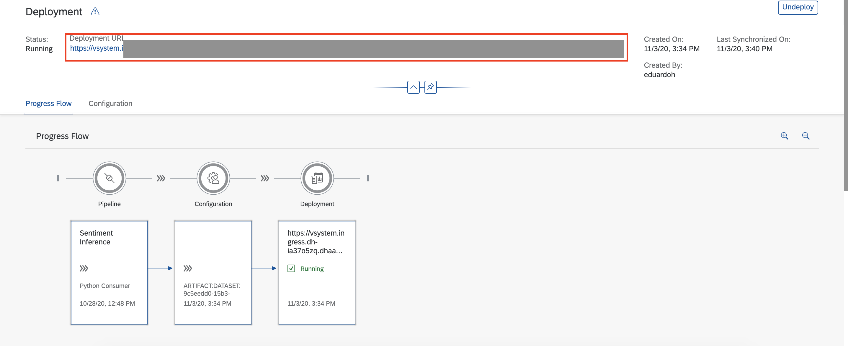
Now, since we will be using POSTMAN to issue the POST request to have the model classify data we send it via JSON, we will be needing the deployment URL which will be available on the top of the same screen. Copy this and head on over to the POSTMAN interface. At this point, I will have to refer you to andreas.forster’s blog post, https://blogs.sap.com/2019/08/14/sap-data-intelligence-create-your-first-ml-scenario/, on deploying a machine learning model with SAP Data Intelligence online with POSTMAN as he covers exactly what steps you need to do to get POSTMAN working. Once, you have put in the necessary parameters, you merely need to write whatever text you want to have classified and click on send to receive the both the classification (as in positive or negative in binary form) as well as the degree of polarity(a float between 0 and 1 determining the degree to how positive or negative the text is) from the deployed model. Now, as the dataset I used was for the review of laptops and computers, I have written:
{
"text": "I thought the computer was amazing and the processor was so fast!"
}

Unsurprisingly, I receive the degree of sentiment which is .999 indicating it to be extremely positive as it is nearly 1 as well as the classification of 1 meaning it is positive. Please remember that Deep Learning models in general will perform best on data which matches that with which it was trained i.e. a review of a laptop for the data I used may get classified well but a Tweet talking about a new song may achieve poor results. Congratulations, we have now built a basic Natural Language Processing model with TensorFlow for sentiment analysis on SAP Data Intelligence. I have tried to keep things as simple as possible so as to ensure that you know the basic infrastructure to develop NLP models on SAP Data Intelligence. What I have described here can be modified tremendously to fit most tasks involving text and deep learning and it is up to your choice as to what you wish to do with it. Nothing is impossible.
Furthermore, I have written another blogpost detailing what values one could derive from sentiment analysis models such as this one which showcases the practical application of such NLP models here, https://blogs.sap.com/2020/12/22/__trashed-31/.
- SAP Managed Tags:
- Machine Learning,
- SAP Data Intelligence,
- Artificial Intelligence,
- SAP Text Analysis
You must be a registered user to add a comment. If you've already registered, sign in. Otherwise, register and sign in.
Labels in this area
-
"automatische backups"
1 -
"regelmäßige sicherung"
1 -
"TypeScript" "Development" "FeedBack"
1 -
505 Technology Updates 53
1 -
ABAP
14 -
ABAP API
1 -
ABAP CDS Views
2 -
ABAP CDS Views - BW Extraction
1 -
ABAP CDS Views - CDC (Change Data Capture)
1 -
ABAP class
2 -
ABAP Cloud
3 -
ABAP Development
5 -
ABAP in Eclipse
1 -
ABAP Platform Trial
1 -
ABAP Programming
2 -
abap technical
1 -
abapGit
1 -
absl
2 -
access data from SAP Datasphere directly from Snowflake
1 -
Access data from SAP datasphere to Qliksense
1 -
Accrual
1 -
action
1 -
adapter modules
1 -
Addon
1 -
Adobe Document Services
1 -
ADS
1 -
ADS Config
1 -
ADS with ABAP
1 -
ADS with Java
1 -
ADT
2 -
Advance Shipping and Receiving
1 -
Advanced Event Mesh
3 -
AEM
1 -
AI
7 -
AI Launchpad
1 -
AI Projects
1 -
AIML
9 -
Alert in Sap analytical cloud
1 -
Amazon S3
1 -
Analytical Dataset
1 -
Analytical Model
1 -
Analytics
1 -
Analyze Workload Data
1 -
annotations
1 -
API
1 -
API and Integration
3 -
API Call
2 -
API security
1 -
Application Architecture
1 -
Application Development
5 -
Application Development for SAP HANA Cloud
3 -
Applications and Business Processes (AP)
1 -
Artificial Intelligence
1 -
Artificial Intelligence (AI)
5 -
Artificial Intelligence (AI) 1 Business Trends 363 Business Trends 8 Digital Transformation with Cloud ERP (DT) 1 Event Information 462 Event Information 15 Expert Insights 114 Expert Insights 76 Life at SAP 418 Life at SAP 1 Product Updates 4
1 -
Artificial Intelligence (AI) blockchain Data & Analytics
1 -
Artificial Intelligence (AI) blockchain Data & Analytics Intelligent Enterprise
1 -
Artificial Intelligence (AI) blockchain Data & Analytics Intelligent Enterprise Oil Gas IoT Exploration Production
1 -
Artificial Intelligence (AI) blockchain Data & Analytics Intelligent Enterprise sustainability responsibility esg social compliance cybersecurity risk
1 -
ASE
1 -
ASR
2 -
ASUG
1 -
Attachments
1 -
Authorisations
1 -
Automating Processes
1 -
Automation
2 -
aws
2 -
Azure
1 -
Azure AI Studio
1 -
Azure API Center
1 -
Azure API Management
1 -
B2B Integration
1 -
Backorder Processing
1 -
Backup
1 -
Backup and Recovery
1 -
Backup schedule
1 -
BADI_MATERIAL_CHECK error message
1 -
Bank
1 -
BAS
1 -
basis
2 -
Basis Monitoring & Tcodes with Key notes
2 -
Batch Management
1 -
BDC
1 -
Best Practice
1 -
bitcoin
1 -
Blockchain
3 -
bodl
1 -
BOP in aATP
1 -
BOP Segments
1 -
BOP Strategies
1 -
BOP Variant
1 -
BPC
1 -
BPC LIVE
1 -
BTP
13 -
BTP Destination
2 -
Business AI
1 -
Business and IT Integration
1 -
Business application stu
1 -
Business Application Studio
1 -
Business Architecture
1 -
Business Communication Services
1 -
Business Continuity
1 -
Business Data Fabric
3 -
Business Fabric
1 -
Business Partner
12 -
Business Partner Master Data
10 -
Business Technology Platform
2 -
Business Trends
4 -
BW4HANA
1 -
CA
1 -
calculation view
1 -
CAP
4 -
Capgemini
1 -
CAPM
1 -
Catalyst for Efficiency: Revolutionizing SAP Integration Suite with Artificial Intelligence (AI) and
1 -
CCMS
2 -
CDQ
12 -
CDS
2 -
Cental Finance
1 -
Certificates
1 -
CFL
1 -
Change Management
1 -
chatbot
1 -
chatgpt
3 -
CL_SALV_TABLE
2 -
Class Runner
1 -
Classrunner
1 -
Cloud ALM Monitoring
1 -
Cloud ALM Operations
1 -
cloud connector
1 -
Cloud Extensibility
1 -
Cloud Foundry
4 -
Cloud Integration
6 -
Cloud Platform Integration
2 -
cloudalm
1 -
communication
1 -
Compensation Information Management
1 -
Compensation Management
1 -
Compliance
1 -
Compound Employee API
1 -
Configuration
1 -
Connectors
1 -
Consolidation Extension for SAP Analytics Cloud
2 -
Control Indicators.
1 -
Controller-Service-Repository pattern
1 -
Conversion
1 -
Cosine similarity
1 -
cryptocurrency
1 -
CSI
1 -
ctms
1 -
Custom chatbot
3 -
Custom Destination Service
1 -
custom fields
1 -
Customer Experience
1 -
Customer Journey
1 -
Customizing
1 -
cyber security
3 -
cybersecurity
1 -
Data
1 -
Data & Analytics
1 -
Data Aging
1 -
Data Analytics
2 -
Data and Analytics (DA)
1 -
Data Archiving
1 -
Data Back-up
1 -
Data Flow
1 -
Data Governance
5 -
Data Integration
2 -
Data Quality
12 -
Data Quality Management
12 -
Data Synchronization
1 -
data transfer
1 -
Data Unleashed
1 -
Data Value
8 -
database tables
1 -
Datasphere
3 -
datenbanksicherung
1 -
dba cockpit
1 -
dbacockpit
1 -
Debugging
2 -
Defender
1 -
Delimiting Pay Components
1 -
Delta Integrations
1 -
Destination
3 -
Destination Service
1 -
Developer extensibility
1 -
Developing with SAP Integration Suite
1 -
Devops
1 -
digital transformation
1 -
Documentation
1 -
Dot Product
1 -
DQM
1 -
dump database
1 -
dump transaction
1 -
e-Invoice
1 -
E4H Conversion
1 -
Eclipse ADT ABAP Development Tools
2 -
edoc
1 -
edocument
1 -
ELA
1 -
Embedded Consolidation
1 -
Embedding
1 -
Embeddings
1 -
Employee Central
1 -
Employee Central Payroll
1 -
Employee Central Time Off
1 -
Employee Information
1 -
Employee Rehires
1 -
Enable Now
1 -
Enable now manager
1 -
endpoint
1 -
Enhancement Request
1 -
Enterprise Architecture
1 -
ESLint
1 -
ETL Business Analytics with SAP Signavio
1 -
Euclidean distance
1 -
Event Dates
1 -
Event Driven Architecture
1 -
Event Mesh
2 -
Event Reason
1 -
EventBasedIntegration
1 -
EWM
1 -
EWM Outbound configuration
1 -
EWM-TM-Integration
1 -
Existing Event Changes
1 -
Expand
1 -
Expert
2 -
Expert Insights
2 -
Exploits
1 -
Fiori
14 -
Fiori Elements
2 -
Fiori SAPUI5
12 -
first-guidance
1 -
Flask
1 -
FTC
1 -
Full Stack
8 -
Funds Management
1 -
gCTS
1 -
General
1 -
Generative AI
1 -
Getting Started
1 -
GitHub
9 -
Grants Management
1 -
groovy
1 -
GTP
1 -
HANA
6 -
HANA Cloud
2 -
Hana Cloud Database Integration
2 -
HANA DB
2 -
HANA XS Advanced
1 -
Historical Events
1 -
home labs
1 -
HowTo
1 -
HR Data Management
1 -
html5
8 -
HTML5 Application
1 -
Identity cards validation
1 -
idm
1 -
Implementation
1 -
input parameter
1 -
instant payments
1 -
Integration
3 -
Integration Advisor
1 -
Integration Architecture
1 -
Integration Center
1 -
Integration Suite
1 -
intelligent enterprise
1 -
iot
1 -
Java
1 -
job
1 -
Job Information Changes
1 -
Job-Related Events
1 -
Job_Event_Information
1 -
joule
4 -
Journal Entries
1 -
Just Ask
1 -
Kerberos for ABAP
8 -
Kerberos for JAVA
8 -
KNN
1 -
Launch Wizard
1 -
Learning Content
2 -
Life at SAP
5 -
lightning
1 -
Linear Regression SAP HANA Cloud
1 -
Loading Indicator
1 -
local tax regulations
1 -
LP
1 -
Machine Learning
2 -
Marketing
1 -
Master Data
3 -
Master Data Management
14 -
Maxdb
2 -
MDG
1 -
MDGM
1 -
MDM
1 -
Message box.
1 -
Messages on RF Device
1 -
Microservices Architecture
1 -
Microsoft Universal Print
1 -
Middleware Solutions
1 -
Migration
5 -
ML Model Development
1 -
Modeling in SAP HANA Cloud
8 -
Monitoring
3 -
MTA
1 -
Multi-Record Scenarios
1 -
Multiple Event Triggers
1 -
Myself Transformation
1 -
Neo
1 -
New Event Creation
1 -
New Feature
1 -
Newcomer
1 -
NodeJS
3 -
ODATA
2 -
OData APIs
1 -
odatav2
1 -
ODATAV4
1 -
ODBC
1 -
ODBC Connection
1 -
Onpremise
1 -
open source
2 -
OpenAI API
1 -
Oracle
1 -
PaPM
1 -
PaPM Dynamic Data Copy through Writer function
1 -
PaPM Remote Call
1 -
PAS-C01
1 -
Pay Component Management
1 -
PGP
1 -
Pickle
1 -
PLANNING ARCHITECTURE
1 -
Popup in Sap analytical cloud
1 -
PostgrSQL
1 -
POSTMAN
1 -
Prettier
1 -
Process Automation
2 -
Product Updates
5 -
PSM
1 -
Public Cloud
1 -
Python
4 -
python library - Document information extraction service
1 -
Qlik
1 -
Qualtrics
1 -
RAP
3 -
RAP BO
2 -
Record Deletion
1 -
Recovery
1 -
recurring payments
1 -
redeply
1 -
Release
1 -
Remote Consumption Model
1 -
Replication Flows
1 -
research
1 -
Resilience
1 -
REST
1 -
REST API
1 -
Retagging Required
1 -
Risk
1 -
Rolling Kernel Switch
1 -
route
1 -
rules
1 -
S4 HANA
1 -
S4 HANA Cloud
1 -
S4 HANA On-Premise
1 -
S4HANA
3 -
S4HANA_OP_2023
2 -
SAC
10 -
SAC PLANNING
9 -
SAP
4 -
SAP ABAP
1 -
SAP Advanced Event Mesh
1 -
SAP AI Core
8 -
SAP AI Launchpad
8 -
SAP Analytic Cloud Compass
1 -
Sap Analytical Cloud
1 -
SAP Analytics Cloud
4 -
SAP Analytics Cloud for Consolidation
3 -
SAP Analytics Cloud Story
1 -
SAP analytics clouds
1 -
SAP API Management
1 -
SAP BAS
1 -
SAP Basis
6 -
SAP BODS
1 -
SAP BODS certification.
1 -
SAP BTP
21 -
SAP BTP Build Work Zone
2 -
SAP BTP Cloud Foundry
6 -
SAP BTP Costing
1 -
SAP BTP CTMS
1 -
SAP BTP Innovation
1 -
SAP BTP Migration Tool
1 -
SAP BTP SDK IOS
1 -
SAP BTPEA
1 -
SAP Build
11 -
SAP Build App
1 -
SAP Build apps
1 -
SAP Build CodeJam
1 -
SAP Build Process Automation
3 -
SAP Build work zone
10 -
SAP Business Objects Platform
1 -
SAP Business Technology
2 -
SAP Business Technology Platform (XP)
1 -
sap bw
1 -
SAP CAP
2 -
SAP CDC
1 -
SAP CDP
1 -
SAP CDS VIEW
1 -
SAP Certification
1 -
SAP Cloud ALM
4 -
SAP Cloud Application Programming Model
1 -
SAP Cloud Integration for Data Services
1 -
SAP cloud platform
8 -
SAP Companion
1 -
SAP CPI
3 -
SAP CPI (Cloud Platform Integration)
2 -
SAP CPI Discover tab
1 -
sap credential store
1 -
SAP Customer Data Cloud
1 -
SAP Customer Data Platform
1 -
SAP Data Intelligence
1 -
SAP Data Migration in Retail Industry
1 -
SAP Data Services
1 -
SAP DATABASE
1 -
SAP Dataspher to Non SAP BI tools
1 -
SAP Datasphere
9 -
SAP DRC
1 -
SAP EWM
1 -
SAP Fiori
3 -
SAP Fiori App Embedding
1 -
Sap Fiori Extension Project Using BAS
1 -
SAP GRC
1 -
SAP HANA
1 -
SAP HCM (Human Capital Management)
1 -
SAP HR Solutions
1 -
SAP IDM
1 -
SAP Integration Suite
9 -
SAP Integrations
4 -
SAP iRPA
2 -
SAP LAGGING AND SLOW
1 -
SAP Learning Class
1 -
SAP Learning Hub
1 -
SAP Master Data
1 -
SAP Odata
2 -
SAP on Azure
2 -
SAP PartnerEdge
1 -
sap partners
1 -
SAP Password Reset
1 -
SAP PO Migration
1 -
SAP Prepackaged Content
1 -
SAP Process Automation
2 -
SAP Process Integration
2 -
SAP Process Orchestration
1 -
SAP S4HANA
2 -
SAP S4HANA Cloud
1 -
SAP S4HANA Cloud for Finance
1 -
SAP S4HANA Cloud private edition
1 -
SAP Sandbox
1 -
SAP STMS
1 -
SAP successfactors
3 -
SAP SuccessFactors HXM Core
1 -
SAP Time
1 -
SAP TM
2 -
SAP Trading Partner Management
1 -
SAP UI5
1 -
SAP Upgrade
1 -
SAP Utilities
1 -
SAP-GUI
8 -
SAP_COM_0276
1 -
SAPBTP
1 -
SAPCPI
1 -
SAPEWM
1 -
sapfirstguidance
1 -
SAPHANAService
1 -
SAPIQ
1 -
sapmentors
1 -
saponaws
2 -
SAPS4HANA
1 -
SAPUI5
5 -
schedule
1 -
Script Operator
1 -
Secure Login Client Setup
8 -
security
9 -
Selenium Testing
1 -
Self Transformation
1 -
Self-Transformation
1 -
SEN
1 -
SEN Manager
1 -
service
1 -
SET_CELL_TYPE
1 -
SET_CELL_TYPE_COLUMN
1 -
SFTP scenario
2 -
Simplex
1 -
Single Sign On
8 -
Singlesource
1 -
SKLearn
1 -
Slow loading
1 -
soap
1 -
Software Development
1 -
SOLMAN
1 -
solman 7.2
2 -
Solution Manager
3 -
sp_dumpdb
1 -
sp_dumptrans
1 -
SQL
1 -
sql script
1 -
SSL
8 -
SSO
8 -
Substring function
1 -
SuccessFactors
1 -
SuccessFactors Platform
1 -
SuccessFactors Time Tracking
1 -
Sybase
1 -
system copy method
1 -
System owner
1 -
Table splitting
1 -
Tax Integration
1 -
Technical article
1 -
Technical articles
1 -
Technology Updates
15 -
Technology Updates
1 -
Technology_Updates
1 -
terraform
1 -
Threats
2 -
Time Collectors
1 -
Time Off
2 -
Time Sheet
1 -
Time Sheet SAP SuccessFactors Time Tracking
1 -
Tips and tricks
2 -
toggle button
1 -
Tools
1 -
Trainings & Certifications
1 -
Transformation Flow
1 -
Transport in SAP BODS
1 -
Transport Management
1 -
TypeScript
3 -
ui designer
1 -
unbind
1 -
Unified Customer Profile
1 -
UPB
1 -
Use of Parameters for Data Copy in PaPM
1 -
User Unlock
1 -
VA02
1 -
Validations
1 -
Vector Database
2 -
Vector Engine
1 -
Visual Studio Code
1 -
VSCode
2 -
VSCode extenions
1 -
Vulnerabilities
1 -
Web SDK
1 -
work zone
1 -
workload
1 -
xsa
1 -
XSA Refresh
1
- « Previous
- Next »
Related Content
- Feature Request: Allow Process Intelligence Consumers to save personal filters in Technology Q&A
- Up Net Working Capital, Up Inventory and Down Efficiency. What to do? in Technology Blogs by SAP
- 10+ ways to reshape your SAP landscape with SAP Business Technology Platform – Blog 4 in Technology Blogs by SAP
- Harnessing the Power of SAP HANA Cloud Vector Engine for Context-Aware LLM Architecture in Technology Blogs by SAP
- UNVEILING THE INNOVATIONS OF ARTIFICIAL INTELLIGENCE in Technology Q&A
Top kudoed authors
| User | Count |
|---|---|
| 9 | |
| 8 | |
| 5 | |
| 5 | |
| 4 | |
| 4 | |
| 4 | |
| 3 | |
| 3 | |
| 3 |