


- SAP Community
- Products and Technology
- Technology
- Technology Blogs by SAP
- Network Performance Analysis for SAP Netweaver ABA...
Technology Blogs by SAP
Learn how to extend and personalize SAP applications. Follow the SAP technology blog for insights into SAP BTP, ABAP, SAP Analytics Cloud, SAP HANA, and more.
Turn on suggestions
Auto-suggest helps you quickly narrow down your search results by suggesting possible matches as you type.
Showing results for
Product and Topic Expert
Options
- Subscribe to RSS Feed
- Mark as New
- Mark as Read
- Bookmark
- Subscribe
- Printer Friendly Page
- Report Inappropriate Content
02-21-2023
10:01 PM
Introduction
Typically, SAP Systems are configured in a three-tier configuration: the presentation tier or layer (FIORI, SAP GUI, or HTML browser), the application layer (SAP Netweaver ABAP/Java), and the storage/database tier.
- The Presentation Tier: This is the user interface layer and is responsible for displaying data to the user and allowing the user to interact with the application. This tier can include web pages, desktop interfaces or mobile apps.
- The Application Tier: This is the middle layer and is responsible for the business logic and data processing. This tier performs tasks such as data validation, calculations, and communicating with the storage tier to retrieve or store data.
- The Storage/Database Tier: This is the bottom layer and is responsible for the permanent storage and retrieval of data. This tier can be implemented using a database management system (DBMS) such as SAP HANA, ASE, MaxDB, DB2, Oracle, or Microsoft SQL Server.
Such a three-tier architecture provides several benefits, including improved scalability, maintainability, and security. By separating the different functions into distinct layers, changes to one layer can be made without affecting the others, making the application more flexible and easier to maintain.
The different layers/tiers and components in a three-tier software architecture communicate with each other using a combination of protocols and APIs. Some common protocols used in three-tier architecture include HTTP, HTTPS, TCP/IP, and message queues. The communication between the tiers typically occurs over a network, such as a local area network (LAN), wide area network (WAN), or the internet.
Content
Network Performance
Network performance is critical in a three-tier software architecture because of the way the different tiers communicate with each other. In this architecture, the presentation tier, the application tier, and the storage tier are often located on different physical or virtual machines, and therefore communicate over a network. This communication is critical for the overall performance and reliability of the application.
If the network is slow or unreliable, it can cause significant delays in the processing of data and lead to slow response times for the user. Additionally, if the network experiences high levels of traffic or congestion, it can cause dropped packets or even complete failures in communication between the tiers. This can result in data loss or corruption, which can have serious consequences for the application and its users.
Therefore, it is important to ensure that the network used in a three-tier architecture has high levels of performance, reliability, and security. This may involve using redundant networks, load balancing, and firewalls to protect against network-based attacks, as well as monitoring network performance and capacity to detect and resolve issues before they become critical.
By investing in a robust network infrastructure, organizations can ensure the performance, scalability, and security of their three-tier applications.
The application tier of an SAP NetWeaver ABAP system is composed of several individual components, including:
- SAP ABAP/JAVA Application Server: This component provides the business logic and data processing capabilities for SAP applications. This Application Server is providing several types of work processes, including dialog processes (for handling user interactions), update processes (for handling database updates), and background processes (for handling batch processing).
- SAP Message Server: This component provides load balancing and failover capabilities for the Application Tier. It distributes incoming requests to the available work processes and can also dynamically allocate work processes based on system load.
- SAP Enqueue Server: This component provides locking and synchronization services for the Application Tier. It ensures that data is updated in a consistent and synchronized manner, even in a multi-user environment.
- SAP Gateway: The SAP Gateway acts as a central hub for managing authentication, authorization, and security for external access to SAP systems.
These various components of those application servers communicate with each other via network using the TCP/IP protocol.

We typically name the network components connecting the users (GUI, Web clients) with the application server as frontend network, the network parts connecting the various component of the application server with each other and the database as backend network.
The performance of this backend network has a high impact on the overall response time – a poor network will significantly increase the database response or enqueue response times. The total DB response time as seen from the dialog work process consists of the network time from the dialog process to the DB, the DB execution time and the time to send the result back to the dialog process.
Especially for HANA customers, which have high expectations to see improved performance compared to their old installations, the network times are very critical; a poor network has the potential to make the very good HANA response times invisible and consequently leading to customer complaints about the HANA related products.
The execution time of a fast DB statement (e.g. select single from table T100) is in the range of 100 μs or even faster. The network time for a fast round trip (SAP > DB > SAP) is typically around 300 μs. The total time for such a fast DB select statement is therefore at approximately 400 μs where the network roundtrip time counts for 75% of the total DB response time. Some customer installations have much higher roundtrip times of more than 700μs which severely impact the total execution time for a SQL statement.

Impact on Response Times
The impact of high network latency can be seen when analyzing the statistical records from transaction STAD. In the below example we see an update process on a system with a high latency of approximately 0.70ms.

The total DB request time was at 65ms for a total of 61 DB requests. If the customer would be able to reduce the latency by 0.3ms, then total time for the 61 database requests would be reduced by approximately 61*0.3ms = 18.3ms. The total DB time therefore be reduced from 65ms to 48ms which is an improvement of 28%. In this example the network time can be estimated at 61*0.7ms = 42ms which is 66% of the total DB time.
To describe the quality of a network we use the following terms:
- Bandwidth: The maximum amount of data that can be transmitted over a network in a given time period, usually measured in bits per second or bytes per second.
- Throughput: The actual amount of data that is transmitted over a network in a given time period, measured in bits per second or bytes per second.
- Latency: The time it takes for a data packet to travel from one point to another in a network, measured in milliseconds. The latency is mainly a function of the signals travel time and processing time at any nodes the information traverses. Additional network infrastructure components like switches, routers, firewalls typically increase this latency.
- Jitter:The variation in packet delay at the receiver of the information
- Error rate: The number of corrupted bits expressed as a percentage or fraction of the total sent
SAP NetWeaver ABAP does not have advanced features for directly evaluating network quality, but there are some tools available that can help determine if the network performance is sufficient.
In this document we describe the following tools to analyze network performance:
- PING/NIPING - measures the round-trip time for messages sent from the originating host to a destination computer that are echoed back to the source.
- ABAPMETER - system performance benchmark/monitoring tool
- Snapshot Monitor - collect system metrics like CPU/MEM usage and NetRTT
- SQL Monitor & Traces – measure execution times of select statements
- RSMONENQ_PERF – analyze enqueue performance
- TCPDUMP – network packet analyzer
For more detailed information about network performance we refer to the following documents:
- Wikipedia Network Performance - https://en.wikipedia.org/wiki/Network_performance
- SAP Note: 1100926 - FAQ: Network performance
- SAP Note:2081065 - Troubleshooting SAP HANA Network
- SAP Note: 2222200 - FAQ: SAP HANA Network
- SAP Note: 500235 - Network Diagnosis with NIPING
Network Layers
The OSI (Open Systems Interconnection) model defines the communication functions and protocols needed for successful data exchange between two end systems in a computer network. Different protocols are used at each layer of the OSI model to achieve this communication. Here is a brief summary of the typical protocols used in each layer:
- Physical Layer: This layer deals with the transmission of individual bits over the physical media. The protocols used in this layer include RS-232, Ethernet, and Wi-Fi.
- Data Link Layer: This layer provides error detection and correction services, as well as flow control to ensure that data is transmitted reliably over the network. The protocols used in this layer include Ethernet, PPP, and FDDI.
- Network Layer: This layer is responsible for routing data packets between networks, as well as addressing and fragmentation of data packets. The protocols used in this layer include IP (Internet Protocol), ICMP (Internet Control Message Protocol), and ARP (Address Resolution Protocol).
- Transport Layer: This layer provides reliable end-to-end communication, including flow control, error correction, and segmentation of data into manageable blocks. The protocols used in this layer include TCP (Transmission Control Protocol) and UDP (User Datagram Protocol).
- Session Layer: This layer provides the means for establishing and maintaining communication between endpoints, as well as synchronization and recovery of the session. The protocols used in this layer include SSL (Secure Sockets Layer) and TLS (Transport Layer Security).
- Presentation Layer: This layer is responsible for data format conversion and encryption, to ensure that data can be easily understood by the receiving system. The protocols used in this layer include ASCII (American Standard Code for Information Interchange), JPEG (Joint Photographic Experts Group), and MPEG (Moving Picture Experts Group).
- Application Layer: This layer provides the interface between the end user and the network, and is responsible for services such as email, file transfer, and printing. The protocols used in this layer include SMTP (Simple Mail Transfer Protocol), FTP (File Transfer Protocol), and HTTP (Hypertext Transfer Protocol).
Note that these protocols are not exhaustive and there are many other protocols that can be used in each layer.
The different network layers/protocols and analysis tools are illustrated below:
Any network analysis on network layers 2 or higher might be impacted by CPU bottlenecks, a very high CPU usage can result in elevated response times which are not related to the physical network itself. It is therefore mandatory to review the CPU usage on both sides in order to rule out that the measurement results are caused by a CPU overload.
PING and NIPING
The most commonly known tools to analyze a network are PING and NIPING. Both are similar but there are differences one should know. In the OSI/ISO network layer model the PING and NIPING work on different network layers. While PING works on level 3 (IP layer) with protocol ICMP, NIPING (which is part of the SAP software on each application server) works on level 4 (Transport layer TCP). The main difference is that NIPING works on a dedicate port and apart from a performance test it also allows to test firewall settings (e.g. test if a port is open or not).

With PING and NIPING we can measure both, the network latency (using very small packages) or the throughput (using very large packages).
Package Size
The impact of the low bandwidth, reduced throughput or high latency on the database performance depends on the type of select statements and the size of the result set which is transferred back from the database to the applications server.
In a typical transactional SAP system most of the select statements transfer packages back from the DB to the application server of only 66 to 900 bytes – around 70% of all DB response fit into a single TCP package of a Maximum Transmission Unit MTU of 1500 bytes. For those small packages send back from the DB, latency is most important as it represents a constant offset in the transmission time. For very large packages the max. achievable throughput will be more important.
To analyze the network latency which is most critical for fast database selects or enqueue requests, one should use small packages, for a throughput or bandwidth measurement very large packages are recommended. For general analysis one normally uses a package size which fits into a single TCP package. Commonly we use 100 to 300 bytes.
PING
A PING test can be executed from within the SAP application server (transactions OS01, ST06) or from the command line on OS level
$> ping 10.54.42.101
The ping result is not very accurate (no decimals available).
Pinging 127.0.0.1 with 32 bytes of data:
Reply from 127.0.0.1: bytes=32 time<1ms TTL=64
Reply from 127.0.0.1: bytes=32 time<1ms TTL=64
Reply from 127.0.0.1: bytes=32 time<1ms TTL=64
Reply from 127.0.0.1: bytes=32 time<1ms TTL=64
Ping statistics for 127.0.0.1:
Packets: Sent = 4, Received = 4, Lost = 0 (0% loss),
Approximate round trip times in milli-seconds:
Minimum = 0ms, Maximum = 0ms, Average = 0ms
Average PING result below 1ms do not necessarily indicate that the times are perfect. The time resolution of PING is not accurate enough. If the average times are above 1ms then a detailed network analysis should be performed using more accurate tools like NIPING or TCPDUMP.
Average PING result below 1ms do not necessarily indicate that the times are perfect. The time resolution of PING is not accurate enough. If the average times are above 1ms then a detailed network analysis should be performed using more accurate tools like NIPING or TCPDUMP.
NIPING
NIPING is a network diagnostic tool that allows you to check the availability and quality of a network connection between two systems. The tool is commonly used to test the connectivity and performance of a network in SAP environments, where network performance is critical to the overall performance of the system.
The NIPING needs to be started in two separate modes:
| NIPING Server: | listening for incoming network packets on a specified port and responds to them |
| NIPING client | sending network packets to a specified destination system, such as a Niping server. The RTT of the packets is measured and the results are displayed, providing information on the quality of the network connection from the source system to the destination system. |
The NIPING command must be executed via command line on both sides, on the target host we first need to start the NIPING server which will receive the NPING client requests and reply back.

On the server side we typically start the NIPING server with the command:
$> niping -s -I 0
-s server mode
-I x idle time
x > 0 shutdown after x seconds
x = 0 no automatic shutdown
x < 0 shutdown after x seconds idle or first client disconnect
On the client side we use a command like:
$> niping -c -H 192.168.201.45 -B 100 -L 86400 -D 1000 -P >> niping.txt
-c client mode
-s server mode
-H <IP-Address> target host
-B sss package size
-D nnn delay between sends
-L number of loops (repetitions)
-P detailed output
More information about how to use NIPING is available via command nipping /? or in SAP notes:
500235 - Network Diagnosis with NIPING.
2986631 - How to do NIPING and checking network performance
The NIPING list output typically looks like:
---------------------------------------------------
trc file: "nipingresult.txt", trc level: 1, release: "753"
---------------------------------------------------
Tue Sep 17 09:22:33 2019
connect to server o.k.
0: 9.339 ms
Tue Sep 17 09:22:34 2019
1: 3.112 ms
Tue Sep 17 09:22:35 2019
2: 0.448 ms
Tue Sep 17 09:22:36 2019
3: 0.843 ms
In order to process the result of a NIPING analysis we recommend using the DA Data Analysis tool which is described and available in SAP note 3169320 Data Analysis.
LAN Traffic: If client and server are within the same data center the times should be as indicated below (see SAP notes 1100926, 2081065 )
- Good value: Roundtrip time <= 0.3 ms
- Moderate value: 0.3 ms < roundtrip time <= 0.7 ms
- Below average value: Roundtrip time > 0.7 m
WAN Traffic: For larger distances one must expect higher NIPING response times. The response times per 100km distance between client and server can be interpreted as indicated below:
- Good value: Roundtrip time <= 1.5 ms / 100km
- Moderate value: 1.5 ms / 100km < roundtrip time <= 2.5 ms / 100km
- Below average value: Roundtrip time > 2.5 ms / 100km

(An example for typical WWAN response times can be found at https://wondernetwork.com/pings/New%20York)
Fluctuations
Even for a very good network or a loopback scenario the standard deviation which describes the average difference between the individual measurements from the overall average value is typically very high and does not allow to judge if the fluctuations are within normal range (the histogram shape is closer to a log-normal distribution).
 | In a typical normal distribution 68,27 % of all measurements are within the standard deviation σ from the mean (Full width at half maximum). Within the NIPING analysis and monitor tool we calculate the percentage of values found within this standard deviation and compare this value against the expected value within a normal distribution. A value of close or more than 100 % indicates that the fluctuations are normal, lower values indicate that the fluctuations are much higher. |
In the below Example we see three different NIPING results for a fast, medium and slow network where we clearly see the differences between the fluctuations in the corresponding histograms.
| Low Fluctuations | Medium Fluctuations | High Fluctuations |

| 
| 
|
In order to ensure that the NIPING result is not impacted by the host server itself we always recommend performing a loopback ping at the same time for comparison. If the loopback result (nipping server and client on the same machine) is showing high fluctuations then the server itself might have a problem like high CPU usage, small IP/TCP buffers…
The statistical errors of any measurement series which is subject to random fluctuations can be estimated by the formula E% = SQRT(n)/n where n is the number of measurements. In order to keep the statistical errors small at less than 5% we recommend having at least 500 measurements.
Good values: peak below 0.50ms ideally at around 0.25 – 0.35ms with less than 10% of all packages exceeding 0.7 seconds
Bad Values: peak above 0.50ms and/or more than 20% of all packages above 0.70ms
ABAPMETER
ABAPMETER is a performance benchmark tool available with every Netweaver ABAP stack system. One can execute ABAPMETER via transaction ST13.

Select PERF_TOOL and execute.

Then select ABAPMETER and execute again.
The result typically example is shown below (for a perfect DB & Network Performance)

ABAPMETER is performing multiple different tests mostly related to CPU/MEM performance but two of those tests (columns Acc.DB and E.Acc.DB) can be used to measure the DB and network performance.
ABAPMETER executes on each application server 200 identical select statements against the message table T100. One of the selects is for an existing message, the second select will try to read a non-existing record. Both select statements specify the full primary key of table T100. The ABAP coding is shown below.

ABAPMETER will show the total execution time for 200 identical select statements.

If ABAPMETER is showing elevated times, then those increased execution times could either result from a poor performing database or from a slow network. To distinguish between the poor DB or network performance we must do an SQL trace on the application server (via ST05, ST12 or SQLM) and compare those results with a trace taken directly on the database or by analyzing the SQL statement cache (via ST04).
As mentioned in the previous section the ideal network response for a roundtrip is at 350 μs (for some very fast networks we even see roundtrip times of only 150us). The DB execution time on HANA for the empty T100 select should be faster than 75 μs. The total execution time measured by ABAPMETER for 200 repetitions are therefore between:
- Good value: ABAPMETER = 200 * (300 + 75) = 75 ms
- Moderate value: ABAPMETER < 200 * (700 + 75) < 155 ms
- Below average value: ABAPMETER > 200 * (700 + 75) > 155 ms
SAP recommends that a value shown by ABAPMETER for the empty DB access of more than 140ms (= 0.70ms per single execution) should be investigated further (see SAP note 2222200).

ABAPMETER will normally be executed in the foreground as online report but it can also be scheduled in the background. The result of each ABAPMETER execution is then saved as individual spool file. One can display and download those spool files via transaction SP01.

Start SP01 and specify the username executing ABAPMETER together with suffix 2 = *CAT*

Now first save this list as local file e.g. SPOOL.TXT (System > List > Save > Local File > unconverted). This data is important because it contains date/time of the execution – the ABAPMETER spool file itself does not contain any date/time information which could be extracted.
Now mark all spool files and select Spool Request > Forward > Export as Text…
Once all files are downloaded follow the instruction of SAP note 2879613 - ABAPMETER in NetWeaver AS ABAP or import the files directly into Data Analysis (see SAP Note 3169320 - Data Analysis)
The tool Data.Analysis.HTML allows to display the data as scatterplot and histogram – simply press the Graphic button to display the data.

Although even a few executions of ABAPMETER give already a first glimpse of the network performance one should execute ABAPMETER in intervals of around 5 minutes over a duration of at least 24h. A better understanding can be achieved if ABAPMENETER data is collected for multiple days. The collected data will then show if the performance is showing regular peaks during daily peak hours and what are the typical fluctuation in those measurements.
Ideally the times should be stable throughout a day with only minor fluctuations of +/- 20% around the peak value in a histogram (average value in scatter plot or bar chart).

In the above example we see some extreme fluctuations. We also see that during the daily peak hours the times are regularly increasing by a factor of 4 and more. This is a typical example which required a more in-depth analysis using the other tools described in this document. Overall the times are bad – most measurements are above the SAP recommended value of 140ms for 200 select statements as indicated by the yellow line, the average execution time red line in the above example was at 170ms.
The points below which seem somehow separated are from the primary application server which is located on the same host machine using no physical network but a VIOS partition to connect to the HANA database server.
Below an example of a perfectly tuned SAP HANA system with only minor fluctuations.
| A perfect example of ABAPMETER with very fast network connection
| If we zoom in, we see only minor fluctuations the average is at only 47ms.
|
Snapshot Monitor
With ST-PI support package 23 or after implementing SAP note 3318669 - Add Network Roundtrip Time RTT to /SDF/SMON we have the possibility to measure the network latency with the snapshot monitor /SDF/SMON (see SAP Snapshot Monitoring tool SAP Note 2651881).
The network round trip time NetRTT is measured on the application layer of the OSI/ISO network communication model by executing an empty SQL statement on client table T000 for a non-existing entry, similar like program /SSA/CAT (ABAPMETER). The SQL statement is executed 10 times to ensure that the table is fully buffered in the various DB caches, only the last of the 10 executions is measured in microseconds. The total response time depends on multiple factors and therefore a non-optimal response time cannot necessarily be attributed to network problems (high CPU usage on the DB or SAP application server can have a negative impact on the response time).
Ideally the response times of this measurements are around 300-400 μs, values over 750 μs should be investigated further with other tools like NIPING.
- Good value: NetRTT <= 350 μs
- Moderate value: 350 μs < NetRTT <= 750 μs
- Below average value: NetRTT > 750 μs
The collected data can either be downloaded via transaction /SDF/SMON or directly extracted from table /SDF/SMON_HEADER. Additionally one can use transaction /SDF/SMON_DISPLAY (see SAP note 3210905 or Blog https://blogs.sap.com/2023/05/11/display-snapshot-monitor-data/) to visualize the Network Round Trip Time directly within the SAPGUI browser as shown in the screenshot below:
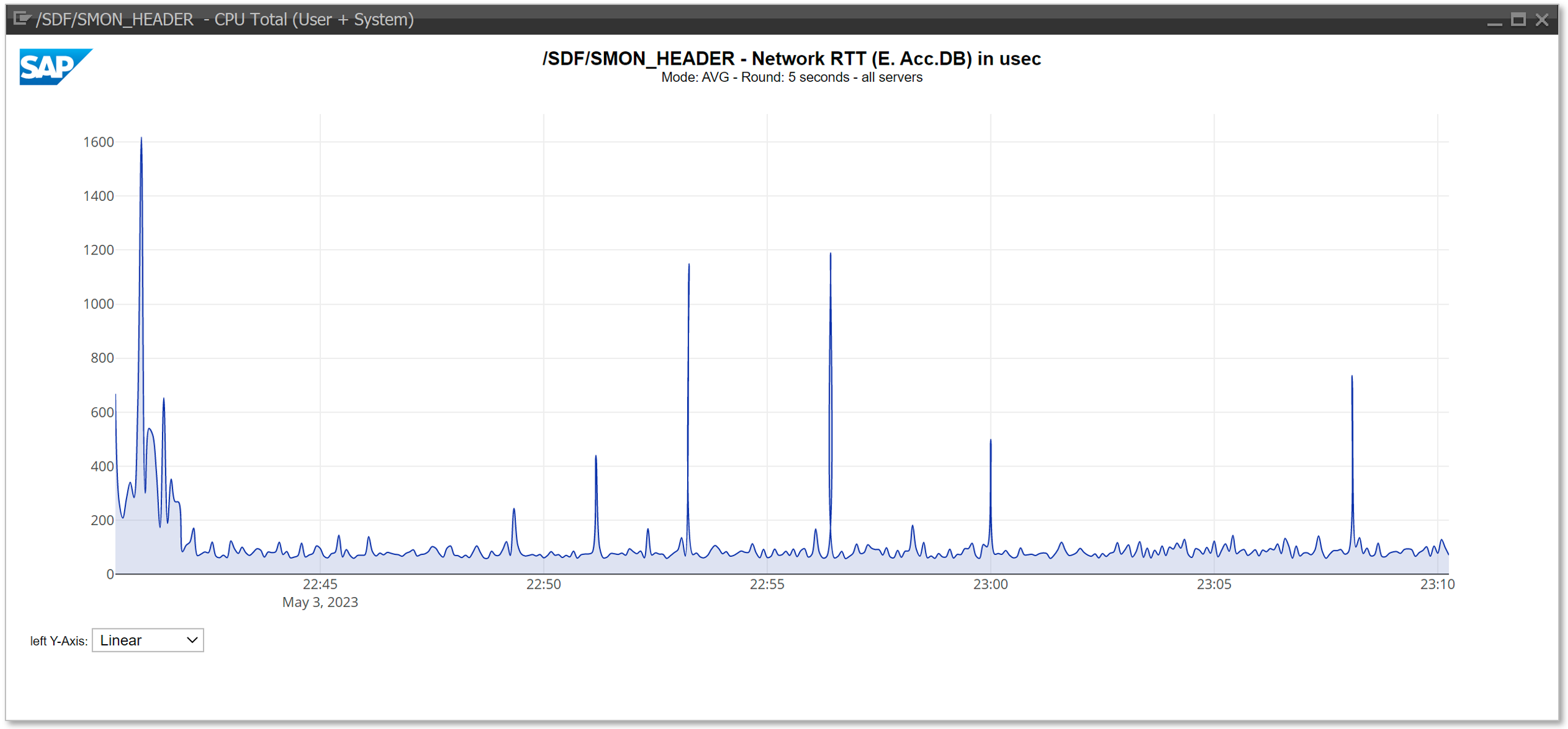
Compared to the NIPING latency measurements (small package size of 100 Bytes) the measured response time NetRTT via /SDF/SMON are typically around 50-80 μs higher.
SQL Traces
We can use SQL traces created from the SAP application server (ST12, ST05) or use the data collected in transaction SQLM (SQL Monitor) to compare the DB execution times measured from the SAP dialog process against the net time measured in the database itself. The difference between these two results can be contributed to the network time. Ideally one should try to trace a select statement which is comparable between different customers. The T100 select statement from ABAPMETER is a perfect candidate but any other fast SELECT SINGLE statement (e.g., from table MAKTX) will work as well. IF the SQL monitor is enabled you don’t need a trace, SQLM has collected all data one will need.
(see https://help.sap.com/viewer/a24970c68fcf4770a64bf9a78e3719e2/7.40.17/en-US/6653101633604f3880f2b9375... or the blog https://blogs.sap.com/2013/11/16/sql-monitor-unleashed/ for more details how to activate SQLM).
ST04 SQL Plan Cache
In the below screenshot we see the statistics from the SQL Plan Cache of a HANA database. Lines 2 and 3 show the times for the T100 select from ABAPMTER, line 3 with 0 number of records shows the statistics for the empty database select for a non-existing message.
The average execution time is very fast (Avg.Cursor Duration) is only 66 us !!!

SQL Monitor SQLM
If we use the SQL monitor (transaction SQLM) to display the statistics for the same select but from an application server perspective which includes the network time the result is very different
On the initial screen of SQLM select Display Data

Then specify the package and table (here package = /SSA/ and table = T100 for the ABAPMETER selects)

An example output is shown below.
In the above example the average execution time as received by the dialog work process on the application server is 1583 us which is 24 times slower or 1500 us longer compared to the time measured directly on the DB.
One can now select the Time Series for this empty select statement and analyze the fluctuations throughout the day.

The minimum average time observed between 02:00:00 and 02:59:59 is 0.535ms, the maximum observed average execution time from 10:00:00 and 10:59:59 is 1.415ms which is 3 times slower.
The average times shown in SQLM are lower than the peak values observed by ABABMETER for individual measurements, because SQLM is calculating an average of 55200 executions over a one-hour duration. The conclusion however is the same, in a customer installation with a perfectly sized network the time should be almost constant with fluctuation no more than 25% during the day. The average execution time for this empty T100 select should be no higher than 0.500ms.
The above time series data from SQLM shown as bar chart is showing the fluctuations during the peak business hours. In the below example the times are above the SAP recommended value of 0.35ms per select statement and during the peak times significantly above the 0.70ms threshold. The time measured in the HANA database was 0.066ms.

Good values: Average SQL execution times measured by SQLM are only about 300us slower than the average execution time measure by the DB.
Bad Values: If the difference between the execution times measured by SQLM and the SQL Plan cache results for a short running execution is more than 0.70ms then the problem should be investigated further. The fluctuations shown in SQLM (hourly averages) should be very low with no more than +/- 10%.
Enqueue Performance Test
The performance of SAP lock requests (enqueues) is especially critical for systems which do mass processing of transactional data – examples are industry solutions for DSD, Retail, Utilities or systems like EWM. Slow enqueue performance can lead to reduced throughput. Apart from optimal settings of the parameters which control the enqueue server a very fast network connection between the application servers to the primary application server is essential.
SAP provides a dedicated tool to analyze the performance of the enqueue server. If there is a very large difference between the enqueue response times between the PAS itself and the other application servers, it is very likely that a poor network performance is the main culprit.
To start the enqueue performance tool you can use transaction SM12. Then enter the OK-code TEST followed by the OK-code DUDEL or you can start the program RSMONENQ_PERF directly via SA38.
If the program RSMONENQ_PERF is not available in the system, please follow SAP note 1320810 - Z_ENQUEUE_PERF.
The program RSMONENQ_PERF is executing various tests on each application server and can take a few minutes to complete. An example output is shown below:
01.10.2019         Program RSMONENQ_PERF                 1
----------------------------------------------------------
**********************************************************
***********  REPORT RSMONENQ_PERF   **********************
************** Version: Version 2.16 *********************
**********************************************************
Execution DATE and TIME:  01.10.2019    19:36:00
Execution in SYSTEM:  PRD
Execution on server:  PAS_PRD_00
Kernel Release:753-324
Standalone Enqueue Server Host:  pas_prd

***********************************************************
****************  CONFIGURATION  **************************
***********************************************************
1.1) Valid values for parameter enque/process_location             OK
1.2) Consistency of enque/process_location.                        OK
1.3) Compare SA enqname and SA Service  on all instances           OK
1.4) Skipped
1.5) enque/table_size should be identical on all servers           OK
     Skipped for enque/process_location = REMOTESA
1.6) How many appservers run ENQ processes?                        OK
     Skipped for enque/process_location = REMOTESA
1.7) More than 3 ENQ processes per instance?                       OK
     Skipped for enque/process_location = REMOTESA
1.8) rdisp/restartable_wp must not include ENQ                     OK
     Skipped for enque/process_location = REMOTESA
1.9) location of enque/backup_file                                 OK
     Skipped for enque/process_location = REMOTESA
1.10) enque/query_comm must not be set                             OK
1.11) enque/force_read_via_rfc must not be set                     OK
1.12) enque/save_key_always different from default                 OK
1.13) enque/sync_dequeall should be identical on all servers       OK
1.14) rdisp/thsend_mode should be identical on all servers         OK

   No severe configuration issues detected.
   Section 1 took  00:00:00  seconds!

***********************************************************
************  ENQUEUE PERFORMANCE  ************************
***********************************************************
   All performance test with         100   Requests!
   All Times in micro seconds if not specified separately

2.1) Performance Test between dispatcher and msg server with ADM Messages!

   to  APP01_PRD_01
      Bytes  ms per req      100    200    500    1ms    2ms    5ms    10ms   >10ms
       458     0,645           0      0     39     48     13      0      0      0
       770     0,577           0      0     50     43      7      0      0      0
     1.290     0,762           0      0     44     40      8      8      0      0
     1.810     1,066           0      0     45     32     11      9      3      0
     2.330     0,820           0      0     28     54     14      3      1      0
     3.370     0,865           0      0     18     59     18      5      0      0
     5.450     0,924           0      0     27     58      9      5      0      1

   to  APP02_PRD_02
      Bytes  ms per req      100    200    500    1ms    2ms    5ms    10ms   >10ms
       458     0,336           0      0     98      2      0      0      0      0
       770     0,329           0      0     96      4      0      0      0      0
     1.290     0,468           0      0     91      5      1      3      0      0
     1.810     1,472           0      0     75      8      5      6      5      1
     2.330     1,699           0      0     79      6      5      6      1      3
     3.370     1,519           0      0     47     20     17      8      5      3
     5.450     0,582           0      0     60     33      6      1      0      0

   to  PAS_PRD_00
      Bytes  ms per req      100    200    500    1ms    2ms    5ms    10ms   >10ms
       458     0,316           0     44     41     12      3      0      0      0
       770     0,235           0     64     33      2      0      1      0      0
     1.290     0,255           0     65     28      4      3      0      0      0
     1.810     0,378           0     57     37      4      0      1      0      1
     2.330     0,222           0     55     44      0      1      0      0      0
     3.370     0,267           0     43     53      3      1      0      0      0
     5.450     0,248           0     39     58      3      0      0      0      0
In the above example we see that the response times on the primary application server PAS_PRD_00 are faster than on the other two application servers but the times on those servers are still within normal range and raise no concern. For a good network connection 90% of the measurement results should be below 1ms. If the times are consistently above 1ms reaching even large counts of 5ms or higher the enqueue performance must be investigated in more detail.
IF high enqueue times are observed on all servers (including the PAS server itself) one should check the parameters and CPU usage of the PAS first and raise an incident if the root cause cannot be detected.
If high enqueue times are only visible on the application servers but not on PAS then we have a strong indication for network issues. We recommend performing further analysis like NIPING/PING between the application servers and PAS to confirm the issue.
Very often those high times appear during times of high system load when the network traffic increases – in any case one should check the overall performance on all involved servers especially CPU/MEM usage and work process availability.
Below an extract from the report RSMONENQ_PERF of a customer facing poor network performance during the business peak hours.
   to  saperp01
      Bytes  ms per req      100    200    500    1ms    2ms    5ms    10ms   >10ms
       458     2,019           0      0      0      5     72     17      5      1
       770     1,878           0      0      0      0     71     28      1      0
     1.290     2,245           0      0      0      0     64     31      5      0
     1.810     2,148           0      0      0      0     63     35      0      2
     2.330     2,503           0      0      0      0     59     31     10      0
     3.370     2,883           0      0      0      0     41     53      5      1
     5.450     2,404           0      0      0      0     45     50      5      0
At the same time the PAS server itself was showing very good results
   to  sappas00
      Bytes  ms per req      100    200    500    1ms    2ms    5ms    10ms   >10ms
       458     2,122           0     99      1      0      0      0      0      0
       770     2,623           0     91      8      1      0      0      0      0
     1.290     2,652           0     85     12      3      0      0      0      0
     1.810     1,733           0     87     13      0      0      0      0      0
     2.330     2,002           0     79     19      2      0      0      0      0
     3.370     2,245           0     64     31      5      0      0      0      0
     5.450     2,408           0     36     51     13      0      0      0      0
Good values: 90% of all measurements below or equal to 1ms on servers different than PAS – the PAS server should be 500us or below.
Bad Values: 90% of all measurements are above 1ms with 20% reaching 5ms or more for servers different than PAS but only if the PAS values are good.
Network Package Analysis
Network package analysis is a valuable tool for network administrators and IT professionals to troubleshoot network connectivity issues. Here are some reasons why and when to use network package analysis: Why to use network package analysis:
- To pinpoint the root cause of network problems
- To identify rogue DHCP servers
- To detect malware
- To monitor bandwidth usage
- To examine security issues
- To learn network protocol internals
When to use network package analysis:
- When there is a network disconnection issue
- When there is a slow network speed issue
- When there is a weak Wi-Fi signal issue
- When there is a physical connectivity issue
- When there is an intermittent network problem
Network package analysis tools like Wireshark and TCPDUMP allow network administrators to capture and analyze network traffic to identify the root cause of network connectivity issues. By analyzing the captured packets, administrators can identify patterns and trends that may indicate network problems and take corrective action to fix the issue. Continuous network monitoring software like Obkio Network Performance Monitoring software can also be used to detect intermittent network problems and identify the cause of the issue.
TCPDUMP is a common packet analyzer that runs under the command line. It allows the user to display TCP/IP and other packets being transmitted or received over a network to which the computer is attached. TCPDUMP works on most Unix-like operating systems: Linux, Solaris, HP-UX 11i, and AIX.
TCPDUMP can print or save selected or all network packages. The output file can then be analyzed with other tools like wireshark.
SAP notes 1370469 - How to perform a TCP trace with Wireshark and 1969914 - Packet scanning tutorial using wireshark are describing how perform such an analysis.
To start tcpdump from a command line please refer to the man pages whichprovide more details on the command syntax. An example is given below.
$> tcpdump -ni eth1 -w /sapmedias/tcpdump.pcap
The amount of data send over a fast ethernet can be very huge. On a 10Gbit line with 10% usage tcpdump will capture around 1.25 Gigabyte very 10 seconds. Typically, such an analysis will be limited to a duration of 30-120 seconds.
Wireshark is a free and open-source packet analyzer. It is used for network troubleshooting, analysis, software and communications protocol development, and education. Wireshark is cross-platform, using the Qt widget toolkit in current releases to implement its user interface, and using pcap to capture packets; it runs on Linux, macOS, BSD, Solaris, some other Unix-like operating systems, and Microsoft Windows. Wireshark can be downloaded from www.wireshark.org
On a windows server one can use wireshark to capture and analyze the traffic, on Unix servers one probably must use tcpdump to capture network packets. Once the packates are captured, copy the pcap file to your computer and start wireshark to open the pcap file.

On the main window one will see the sequence number of the captured package, the time stamp, source/target IP addresses, protocol, length of the package in Byte, and additional information like port numbers… If wireshark detects problems (in the above example duplicate ACK acknowledge packages) they will be highlighted.
Wireshark is fully documented – see documentation at www.wireshark.org/docs
Among the several features available in wireshark we list here a few of the most interesting ones:
Follow the TCP stream and see the full communication between App.Server and DB

Packet Length statistics

Endpoint statistics (who was talking with whom – IP-address, Ports, bytes transferred)

Conversations (when did a conversation start)

IO Statistics (bandwidth usage)

The above graph was taken on a server connected with a 10Gbit network – the bandwidth limit is here 1E10 – the 1sec averages were at around 22.5% of the max. capacity.
IO statistics can be produced in different time intervals 1h, 1min, 10sec, 1sec, 100ms, 10ms, 1ms below the same data in 1ms intervals – here the 10Gbit/sec bandwidth translates down to 1E7 bit/ms. We see that in 1ms intervals the network reached 75% of the available bandwidth.

Filters and different color coding can be applied to the IO statistics – in the above example the blue dots are for the src IP = 172… (sending packages of the server were tcpdump was taken, the orange dots are the incoming traffic for the dst IP = ...
Filters and error analysis
One can apply several filters in wireshark to only display various errors:
ICMP errors: icmp.type == 3 || icmp.type == 11
TCP errors: tcp.analysis.flags
Connection Resets: tcp.flags.reset == 1
Filter for IP: ip.addr == x.x.x.x

The various filters can also be applied to all statistics shown earlier.

in the above example we find 72193 packages in TCP Dup ACK error, with a total of 3174948 packages we have 2.3% errors which is very high.
Export Data to Excel
tcpdump data can be exported into CSV files for further analysis. File > Export Package Dissections > As CSV…

one can select if all data capture or displayed/filtered should be exported and the range of packages. (excel can only handle up to 1048576 rows).
Network Disconnections
Analyzing network disconnections can be done in several ways. Here are some steps and tools that can be used:
- Conduct a network stability test: This can be done using tools like Ping and Tracert, which are free and easy to use
- Use a continuous network monitoring software: This is the most accurate way to detect intermittent network problems.
- Capture the network traffic: Using TCPDUMP or Wireshark you can capture the traffic itself and analyze the packages.
To detect the root cause of network disconnections using TCPDUMP and/or Wireshark, you can follow these steps:
- Install TCPDUMP and/or Wireshark: TCPDUMP is a command-line packet analyzer, while Wireshark provides a graphical interface. Install either or both tools depending on your preference and the operating system you are using.
- Capture network traffic: Start capturing network traffic using either TCPDUMP or Wireshark. Both tools allow you to specify network interfaces to capture packets from. For example, if you're experiencing network disconnections on a specific interface, you can capture traffic on that interface only.
Using TCPDUMP: Open a terminal and run the following command:
tcpdump -i <interface> -s 0 -w <output_file.pcap>
Replace <interface> with the network interface you want to capture from (e.g., eth0) and <output_file.pcap> with the desired name of the output capture file.
Using Wireshark: Launch Wireshark and select the appropriate network interface to capture packets from.
- Reproduce the network disconnection: While capturing packets, reproduce the network disconnection issue you're facing. This could involve performing actions that consistently trigger the disconnection or waiting for the disconnection to occur naturally.
- Stop the packet capture: Once you've reproduced the issue or collected enough packets, stop the packet capture in TCPDUMP or Wireshark.
- Analyze the captured packets: Open the captured packet capture file in Wireshark or use the captured file directly with TCPDUMP for analysis. Here are some steps you can take to narrow down the root cause:
Look for TCP retransmissions or out-of-order packets, which could indicate network congestion or packet loss.
Analyze the TCP handshake and check for any anomalies or errors during the establishment of the connection.
Examine the IP and MAC addresses involved to ensure there are no issues with the network configuration or addressing.
Look for any error messages or abnormal behavior in the captured packets that could point to a specific network device or protocol causing the disconnection.
Pay attention to any ICMP (Internet Control Message Protocol) messages, as they can provide insights into network errors or communication issues.
- Search for patterns: Identify any common patterns or anomalies in the captured packets that coincide with the network disconnections. This could include specific error messages, protocol-related issues, or recurring patterns of packet loss or latency.
- Further investigation and troubleshooting: Based on your analysis, you may need to investigate specific network devices, configurations, or protocols that seem to be related to the disconnections. Consult relevant documentation or seek assistance from network administrators or support teams to address the root cause.
Overall, TCPDUMP and Wireshark are powerful tools for network analysis, allowing you to capture and analyze network traffic at a granular level, which can be helpful for troubleshooting network issues, identifying security threats, and optimizing network performance.
Documentation of Network Infrastructure
Network administrators often find themselves grappling with complex configurations, intricate interconnections, and evolving technologies. To streamline this process and enhance the efficiency of troubleshooting, one vital aspect that should not be overlooked is the proper documentation of the network infrastructure. In this section, we will explore the significance of network documentation and discuss the key components that should be included.
A proper documentation of the network infrastructure should include:
- Network topology diagrams illustrating the physical and logical layout of the network.
- Inventory of network devices, including routers, switches, firewalls, and access points, along with their configurations and firmware versions.
- IP addressing scheme, subnets, VLANs, and DHCP configurations.
- Network protocols and routing tables.
- Security measures, including firewall rules, access control lists (ACLs), and VPN configurations.
- Network services and applications running on the network.
- Backup and disaster recovery procedures.
- Network performance metrics and monitoring configurations.
- Contact information for vendors, service providers, and key personnel.
A comprehensive documentation of the used network infrastructure serves various purposes - below a short list describing why a proper network documentation is required:
- Network Understanding: Documentation serves as a comprehensive reference for understanding the network infrastructure. It provides an overview of the network's design, components, and their interconnections, allowing network administrators to grasp the system's intricacies.
- Troubleshooting and Maintenance: Accurate documentation is invaluable when troubleshooting network issues or performing maintenance tasks. It helps network administrators identify the physical and logical layout of the network, locate specific devices, and understand their configurations, reducing downtime and minimizing the time required for resolution.
- Network Planning and Expansion: Documentation plays a crucial role in network planning and expansion efforts. By documenting the existing network infrastructure, administrators can identify potential areas for improvement, such as capacity constraints, outdated equipment, or inefficient configurations. This information helps in designing and implementing network upgrades or expansions.
- Change Management: Networks evolve over time with modifications, upgrades, and new additions. Proper documentation enables effective change management by providing a historical record of network changes, including device configurations, IP addresses, subnet masks, VLANs, and routing protocols. It helps track changes, verify the network's state before and after modifications, and aids in rollback procedures if needed.
- Security and Compliance: Network documentation is crucial for ensuring security and compliance with regulatory standards. By documenting the network's topology, security measures, access controls, and device configurations, administrators can identify potential vulnerabilities, assess risks, and implement appropriate security measures. Documentation also aids in demonstrating compliance with industry regulations and best practices.
- Disaster Recovery and Business Continuity: In the event of a network outage or disaster, having up-to-date documentation becomes vital. It assists in identifying critical components, backup configurations, and recovery procedures, enabling faster restoration of network services and minimizing business disruption.
Below some examples for network diagrams
 |  |
| (Diagram Examples from https://www.edrawsoft.com/topology-diagram-example.html) |
Network Tuning
Reducing network latency between a database server and an application server is crucial for improving performance and responsiveness. Here are several recommendations that a network expert might suggest:
Physical Proximity: Locate the database server and application server in the same data center or as close to each other as possible. The physical distance between servers can significantly impact latency, as signals need less time to travel shorter distances.
Network Infrastructure Upgrades:
- High-Speed Networking Hardware: Use high-quality, enterprise-grade networking equipment, including switches and routers that can handle high throughput and low latency.
- Fiber Optic Cables: Replace older copper cables with fiber optic cables where possible, as fiber offers higher speeds and lower latency.
Direct Connections: Establish a direct connection between the servers, avoiding any unnecessary hops or intermediaries that can add delay.
Optimized Routing: Implement advanced routing protocols that dynamically find the fastest path for data packets between servers.
Quality of Service (QoS): Configure QoS on network devices to prioritize traffic between the database and application servers. This ensures that critical data isn't delayed by less sensitive traffic.
Network Interface Cards (NICs): Use multi-gigabit or 10 Gigabit NICs that can reduce transmission time and handle higher loads with lower latency.
Reduce Network Traffic: Limit the amount of non-essential traffic on the network segment used by the database and application servers. This can be achieved by network segmentation or Virtual LANs (VLANs).
Server and Network Tuning:
- TCP/IP Stack Optimization: Adjust the server's TCP stack settings (such as window size and buffer settings) to optimize data flow.
- Database Queries Optimization: Optimize the queries to reduce the data transferred between the database and application servers.
Load Balancers: Use load balancers that can intelligently direct traffic and reduce the load on individual servers, thereby potentially reducing response times.
Use of Content Delivery Networks (CDNs): While more relevant for web content, in some architectures, CDNs or similar technologies might be used to cache database queries and results at network edges closer to where they are needed.
Monitoring and Regular Audits: Continuously monitor network performance and conduct regular audits to find and mitigate any new issues that might cause increased latency.
Implementing these strategies involves both hardware upgrades and software configurations, and the specific choices would depend on the existing infrastructure, budget, and criticality of the application.
Proximity Placement
To minimize network latency, improve application performance, and increase the reliability of distributed systems many cloud service providers like Azure, AWS, GCP offer the concept of proximity placement. Each major cloud service provider has its strategies and tools to manage this concept, although the specific features and names might differ. Here’s an overview of how proximity placement is handled by Azure, AWS, and Google Cloud Platform (GCP).
Azure: Proximity Placement Groups
Azure provides a feature called Proximity Placement Groups (PPGs) to help achieve lower latency and higher throughput between deployed resources. This is particularly useful when deploying resources that need to communicate with each other frequently or require low network latency, such as SAP HANA databases or other high-performance computing scenarios.
- Purpose: PPGs ensure that Azure resources like VMs, Virtual Machine Scale Sets, and Azure Dedicated Hosts are physically located close to each other within a single data center or within nearby data centers.
- Use Cases: Ideal for scenarios requiring tight network integration between resources, like clustered databases, high-performance computing, and real-time data processing.
AWS: Placement Groups
AWS offers several types of placement groups that dictate how instances are positioned within the underlying hardware to optimize performance.
- Cluster Placement Groups: These groups place instances close to each other inside a single Availability Zone. This arrangement minimizes the network latency due to the short physical distance between instances, suitable for high-performance computing (HPC) applications.
- Partition Placement Groups: These groups spread instances across logical partitions, ensuring that groups of instances are isolated from each other. This is useful for workloads that need to be spread across distinct hardware to reduce correlated failures.
- Spread Placement Groups: These place instances on distinct underlying hardware to reduce shared risk among instances. It’s useful for applications that require high availability by reducing the risk of simultaneous failures.
Google Cloud Platform (GCP): Resource Locations
Within GCP you can create the following types of placement policies:
Compact placement policy: This policy specifies that VMs are placed close together to reduce network latency. Placing your VMs closer to each other is useful when your VMs need to communicate often among each other, such as when running high-performance computing (HPC), machine learning (ML), or database server workloads.
Spread placement policy: This policy specifies that VMs are placed on separate, discrete hardware—called availability domains—for improved availability and reliability. Placing your VMs on separate availability domains helps to keep your most critical VMs running during live migrations of VMs, or reduce the impact of hardware failure among VMs that share the same hardware.
Further Documentation and Links
a list of further links, SAP notes and books about network is provided below:
- An Introduction to Computer Network
https://intronetworks.cs.luc.edu/current1/uhtml/index.html - Display Snapshot Monitor Data | SAP Blogs
https://blogs.sap.com/2023/05/11/display-snapshot-monitor-data/ - Optimum Network Utilization - Network Design - Cisco Certified Expert (ccexpert.us)
https://www.ccexpert.us/network-design-2/optimum-network-utilization.html - SAP Note 500235 - Network Diagnosis with NIPING
https://me.sap.com/notes/500235 - SAP Note 2986631 - How to do NIPING and checking network performance
https://me.sap.com/notes/2986631 - SAP Note 1100926 - FAQ: Network performance
https://me.sap.com/notes/1100926 - SAP Note 2081065 - Troubleshooting SAP HANA Network
https://me.sap.com/notes/ - Global Ping Statistics → New York
https://wondernetwork.com/pings/New+York - SQL Monitor Unleashed | SAP Blogs
https://blogs.sap.com/2013/11/16/sql-monitor-unleashed/ - Wireshark Wiki
https://wiki.wireshark.org/Home
BOOKS:
- The TCP/IP Tutorial and Technical Overview, Adolfo Rodriguez, John Gatrell, John Karas, Roland Pesch...
- TCP/IP Illustrated, Volume 1 (The Protocols), W. Richard Stevens, Addison-Wesley Professional Computing Series, 1994, ISBN 978-0201633467
Conclusion
Network performance analysis is an essential part of managing SAP landscapes to guarantee that the systems will comply with the performance KPIs. Regular network analysis helps to optimize network performance by identifying bandwidth bottlenecks, inefficient protocols, or misconfigured devices. By analyzing network traffic, one can optimize network settings, prioritize traffic, or upgrade hardware to improve network performance.
If any of the above tests will show a non-optimal result on a regular basis (e.g., daily during peak business times) one should involve network experts to investigate the root cause to mitigate the problem.
Let's use the following analogy: network traffic = traffic on a motorway. With the above tools one can measure the average time from for example Frankfurt to Walldorf (latency). Typical times for the 91km trip are around 58 minutes. If we measure significant higher times, then we can conclude that something is wrong, but we do not know what is causing the problem. If the average times are at 2hours or more, than there might be an accident, a construction area with speed limit or just congestion. The above tools like NIPING, ABAPMETER, SQL traces… only allow us to detect if there is a problem, but these tools will not tell us the root cause. For a root cause analysis, a network specialist needs to be involved who will use more sophisticated tools.
In addition to the above tests with PING/NIPING, ABAPMETER, SQL-Analysis, TCPDUMP one needs to have visibility of the network infrastructure in detail.
- How are the different servers connected, which network components are used (network cards, switches, routers, cables, firewalls)?
- Are the involved servers virtualized and are virtual adapters used?
- Is the customer using VLANs and any traffic shaping?
- Additionally, the CPU/MEM usage of the servers is an important aspect – on a database or application server with very high CPU usage many of the above tests will show poor results.
Once the network infrastructure and components are documented, the network relevant parameters on operating system level but also on SAP application and database level must be verified.
Hope you find the blog helpful - stay tuned for further information and updates.
Labels:
10 Comments
You must be a registered user to add a comment. If you've already registered, sign in. Otherwise, register and sign in.
Labels in this area
-
ABAP CDS Views - CDC (Change Data Capture)
2 -
AI
1 -
Analyze Workload Data
1 -
BTP
1 -
Business and IT Integration
2 -
Business application stu
1 -
Business Technology Platform
1 -
Business Trends
1,658 -
Business Trends
93 -
CAP
1 -
cf
1 -
Cloud Foundry
1 -
Confluent
1 -
Customer COE Basics and Fundamentals
1 -
Customer COE Latest and Greatest
3 -
Customer Data Browser app
1 -
Data Analysis Tool
1 -
data migration
1 -
data transfer
1 -
Datasphere
2 -
Event Information
1,400 -
Event Information
67 -
Expert
1 -
Expert Insights
177 -
Expert Insights
301 -
General
1 -
Google cloud
1 -
Google Next'24
1 -
GraphQL
1 -
Kafka
1 -
Life at SAP
780 -
Life at SAP
13 -
Migrate your Data App
1 -
MTA
1 -
Network Performance Analysis
1 -
NodeJS
1 -
PDF
1 -
POC
1 -
Product Updates
4,577 -
Product Updates
346 -
Replication Flow
1 -
REST API
1 -
RisewithSAP
1 -
SAP BTP
1 -
SAP BTP Cloud Foundry
1 -
SAP Cloud ALM
1 -
SAP Cloud Application Programming Model
1 -
SAP Datasphere
2 -
SAP S4HANA Cloud
1 -
SAP S4HANA Migration Cockpit
1 -
Technology Updates
6,873 -
Technology Updates
430 -
Workload Fluctuations
1
Related Content
- Quick & Easy Datasphere - When to use Data Flow, Transformation Flow, SQL View? in Technology Blogs by Members
- Start page of SAP Signavio Process Insights, discovery edition, the 4 pillars and documentation in Technology Blogs by SAP
- Analyze Expensive ABAP Workload in the Cloud with Work Process Sampling in Technology Blogs by SAP
- Introducing Blog Series of SAP Signavio Process Insights, discovery edition – An in-depth exploratio in Technology Blogs by SAP
- Unify your process and task mining insights: How SAP UEM by Knoa integrates with SAP Signavio in Technology Blogs by SAP
Top kudoed authors
| User | Count |
|---|---|
| 28 | |
| 17 | |
| 15 | |
| 13 | |
| 11 | |
| 9 | |
| 8 | |
| 8 | |
| 8 | |
| 7 |