
- SAP Community
- Products and Technology
- Technology
- Technology Blogs by SAP
- HOW TO use the SAP Business Technology Platform to...
Technology Blogs by SAP
Learn how to extend and personalize SAP applications. Follow the SAP technology blog for insights into SAP BTP, ABAP, SAP Analytics Cloud, SAP HANA, and more.
Turn on suggestions
Auto-suggest helps you quickly narrow down your search results by suggesting possible matches as you type.
Showing results for
Product and Topic Expert
Options
- Subscribe to RSS Feed
- Mark as New
- Mark as Read
- Bookmark
- Subscribe
- Printer Friendly Page
- Report Inappropriate Content
01-11-2022
10:11 AM
See HOW Machine Learning on the SAP Business Technology Platform can be used to extend SAP Marketing Cloud with Predictive Scores. WHY we think that this important, will be described in a separate blog that will be published soon by carsten.heuer1. Stay tuned...
As an example of that extensibility, this blog explains how to predict whether a known contact, that is stored in SAP Marketing Cloud, will carry out their first purchase in the next 30 days. The same approach and components of the SAP Business Technology Platform can be used for many other purposes, whether with SAP Marketing Cloud or other Line of Business applications.
In this blog we use a light-weight architecture, using SAP Data Warehouse Cloud in combination with Cloud Foundry. In case you are already using SAP Data Intelligence, which is a comprehensive platform for data orchestration and governance, there would be no need for Cloud Foundry for instance.
This write up is aimed mostly at IT Experts and Data Scientists, who would set this scenario up for end users of SAP Marketing Cloud.
We will look the different steps of this process, how the SAP Business Technology platform extends and complements SAP Marketing Cloud to close this circle.
This blog describes the implementation steps of a full project, that was set up in tight cooperation with carsten.heuer1. What was intended first as a technical overview became a lot more granular than envisioned initially, as there were a lot of details that seemed relevant to be included. A big shout out goes to the great colleagues that helped the project along. fcolombo, abdullah.amerk, kedarnath_ellendula and johannes.hirling and Sven Gilg with the API of SAP Marketing Cloud. nidhi.sawhney, ian.henry and axel.meier with SAP Data Warehouse Cloud. marc.daniau and raymond.yao with the Machine Learning. carlos.roggan and oliver.heinrich with the Job Scheduling Service.
Direct access to the data in SAP Marketing Cloud is not possible, as this could endanger the stability of the solution. Therefore the data needed for our use case needs to be extracted.
SAP Marketing Cloud supports extraction through SAP Smart Data Integration (SDI) and SAP Data Intelligence. Since SAP Data Warehouse Cloud makes use of that supported SDI to access SAP Marketing Cloud, leveraging the Cloud Data Integration adapter, we stay supported by extracting through SAP Data Warehouse Cloud.
SAP Data Warehouse Cloud gives you two options for extracting the data from SAP Marketing Cloud
With the large data volume typically held in SAP Marketing Cloud, we go with the Real-time replication, to avoid having to run full loads repeatedly. Once real-time replication is set up, the system takes care of everything, you will always have the latest data in the SAP Data Warehouse Cloud for Machine Learning, or any other purpose.
So what's required to set up real-time replication?
By the way, before starting to use SAP Data Warehouse Cloud. The use of Machine Learning in SAP Data Warehouse Cloud requires the Script Server. SAP Note 2994416 explains how to request this. Please note that this Script Server requires 3 virtual CPUs. Since the SAP Data Warehouse Trial only contains 2 of these, the trial cannot be used to implement the full scenario.
You may want to create a new space in SAP Data Warehouse Cloud for this project. The space in the screenshots on this blog is called "SAP Marketing Cloud ML". Use the above details to add a connection of type "SAP Marketing Cloud" to your space.
Enter the credentials of the communication arrangement and select the Data Provisioning Agent, which is needed for the real-time replication.
For the Machine Learning part, we want to know two things about our contacts
Especially the interactions, which can be very diverse, will be important for the Machine Learning. They might describe how a contact responded to a campaign (emails opened, emails clicked, mobile push notifications opened or clicked) or how they behaved on your website (website visits, product pages viewed, videos viewed or downloaded, event registrations, document downloaded ...). Details from other applications like Sales Cloud or SAP Commerce Cloud can also be collected by SAP Marketing Cloud and added to the interactions (for instance lead status, opportunity status, sales orders, shopping carts abandoned / checked-out... ). All these activities are called Interactions and the kind of activity is called ‘Interaction Type’ in SAP Marketing Cloud.
Replicating the data of a CDS View in real-time by creating a Graphical View in SAP Data Warehouse. This creates a Remote Table as well as the view. The Remote Table is then configured so that is loads and stores the data physically and updates it in real-time.
The following steps show how to create such a replicated table based on I_MKT_CONTACT. You need to implement the same steps for I_MKT_INTERACTION.
In SAP Data Warehouse Cloud's Data Builder create a new Graphical View. Go to the "Sources" tab and open the connection you had just created to SAP Marketing Cloud. That screen shows up to 1000 CDS views in the ABAP_CDS folder. The two views we require might appear here if your user has access to more than a 1000 views. If that's the case, just click the little icon next to the name of the connection to open a search interface.
Search for: I_MKT_CONTACT. Select it in the folder structure on the left. This will show the Technical Name "MasterData" on the right hand side. Select this name and continue with "Next".
On the next screen enter the names for the Remote Table that is being created. I went with T_I_MKT_CONTACT for both business and technical name. Continue with "Import and Deploy". The Graphical View opens. Set the view's name to "V_I_MKT_CONTACT" and active "Expose for Consumption". It needs to be exposed so that it is accessible from Python. Save and deploy the view.
Similarly, create a graphical view and remote table for the CDS view I_MKT_INTERACTION. Only small difference is that the default name for its table is "Facts", instead of "MasterData".
To have the data actually replicated, just go to the "Data Integration Monitor". Select the table and in the "Table Replication" drop-down chose "Enable Real-Time Access". Set this up for both tables, and that's all! The data gets replicated in real-time. Transferring 20 million records took my system about 4 hours.
The Space Management's Monitor shows how many rows have already been loaded into the tables of type Disk. A quick test for the real-time replication would be to add a new contact in SAP Marketing Cloud, if you are working with a test tenant. This should show up within a few seconds in SAP Data Warehouse Cloud. You have to enter an email address and make sure that this email is not yet in the system. Duplicate contacts are not returned by I_MKT_CONTACT, so it won't be loaded to SAP Data Warehouse Cloud.
Comment on SAP Data Intelligence: In case you are working with SAP Data Intelligence to extract the data from SAP Marketing Cloud, you can use the "Cloud Data Integration" operator.
The detailed interaction data is now accessible for Machine Learning in SAP Data Warehouse Cloud. However, it still needs to be further prepared to be suitable for Machine Learning. We intend to predict whether a known contact, who has never purchased anything so far, will carry out their first purchase.
This is only an example of course, you could use Machine Learning for many other scenarios. Note that the event you want to predict, must already have happened to other contacts in the past. A rough rule of thumb for using the Automated Predictive Library is that these should have occurred about 300 times in the past to find a stable Machine Learning model.
Back to our case. We pretend that today is 1 October 2021, and we want to predict which contacts makes their first purchase in the next 30 days. We can achieve this by training a model on contacts who had made their first purchase in the last 30 days. This means:

Then this trained Machine Learning model will be applied on a similar dataset, using the current date (1 October 2021) as reference. With the current date as reference, the data will be filtered to include only contacts who have never purchased anything. The Machine Learning model then estimates the probability of a person making their first purchase in the future 30 days.
If this time travel sounds odd, it's just learning from the known past (who did make their purchase in the next 30 days as seen from a reference date) to predict today's unknown future.
The "Python Client API for machine learning algorithms" (or in short: hana_ml) will help us create such a view of our contacts. The view will be saved in SAP Data Warehouse Cloud. Even though you are using Python, the data will stay in the SAP Data Warehouse Cloud, where the data will also be processed. In case you haven't used this library so far, I suggest to have a look at wei.han7's blog SAP BTP Data & Analytics Showcase – Empower Data Scientist with Flexibility in an End-to-End Way. That hana_ml library works well with SAP Data Warehouse Cloud, but it can also be used with SAP HANA Cloud or an on-premise SAP HANA.
To build that view which describes the different contacts, you must create a "Database User" in the "Space Management" to access the data from Python.
I named the user DWCUSER. You have to:
When the user is created, you need the host name, the port (always 443) and the password, which is automatically created.
Start the local Python development environment of your choice. I am using Jupyter Notebooks, that were installed through Anaconda. Install the hana_ml library.
As a quick test, you can check the connection from your Python environment to the SAP Data Warehouse Cloud by hardcoding the logon credentials. If this code is failing, check that SAP Datawarehouse Cloud is allowing access to your IP address.
If the above test worked, store the password securely in the hdbuserstore application, which is part of the SAP HANA client. The Hands-On Tutorial: Machine Learning push-down to SAP HANA with Python describes this in a little more detail, but the credentials are stored with:
C:\Program Files\SAP\hdbclient>hdbuserstore -i SET DWC_SMC "YOURHOSTNAME":443 SAPMARKETINGCLOUDML#DWCUSER
The logon can then simply refer to those stored credentials.
Comment on SAP Data Intelligence: If you were using SAP Data Intelligence, the logon credentials would be saved in a connection in SAP Data Intelligence. Python would be scripted in Jupyter Notebooks within a Machine Learning Scenario. A local Python installation would not be required.
First you may want to explore the data. Take a peek at a few rows.
Or count for instance how often the different interaction types occur. Here the 10 most frequent are displayed. It's a demo system with fake data, most sent emails bounced.
Now we need to build the data set for the Machine Learning model, filtered and aggregated as described at the beginning of this chapter. You can be very creative in this step, particularly in creating columns that describe the contacts' past behaviour. In this example we look at a few select activities such as web site visits and searches on the website. To make this most relevant for our business scenario (purchase in the following 30 days), we count how many of these interactions a person had in the 30 days before the reference date, how many in another 30 day period further back (so days 60 to 31 before the reference date) and how the behaviour changed between these two time periods.
Identify the contacts who had not purchased anything by the specified date and create a flag to indicate, whether they did purchase in the following 30 days. That flag will be the target of the Machine Learning model. For now we are hardcoding the 1st of September 2021. Later on we will turn this into a parameter, for which you can specify any date. We will also reduce the dataset to contain only contacts who had an interaction with us in the past 180 days.
Next we need to describe these contacts, who they are and how they behaved in the time before the chosen date. You could potentially add demographic data such as gender or language from the I_MKT_CONTACT provider. However, there is a risk to introduce an unethical bias. You would have to make sure that using such information is suitable in your case. If you have decided you can use such demographic data, then enrich your contact with the following code. In this blog, we decided not to make use of any such data and the 'LanguageCode' from the following example will not be used.
In this blog, the contacts are only described through calculated columns that reflect their interactions. These columns will be used as predictors in the Machine Learning model. Create multiple sets of predictors that will be joined later on.
Our contacts' behaviour 30 days before the chosen date:
Their behaviour in the 30 days further back in the past:
Join the columns of those two subsequent 30 day periods:
Many of these columns show null values. If a person didn't visit the website, there is nothing to count and the result is a null value. Change those null values to numerical zeros.
Calculate further information, how the behaviour changed between those two periods. If a person becomes more active on your website for instance, this could be a good indicator for the intend to purchase a product.
Carry out some tidy ups.
Have a look at the contents of the columns. Depending on your data volume, this could take a few minutes.
We have the customer view, but we want this parameterised, so that you can easily specify the date around which the logic builds up. Use the SELECT statement that the hana_ml library created for the above view, to create the SQL syntax that creates a parameterised view. The hardcoded date of 1 September 2021 becomes a parameter called P_REFERENCEDATE.
Execute the SQL code and you have the view, which can be used both for training the model and applying the model by passing different reference dates as parameter.
As a quick test, call the view with a different reference date and look at a few rows.
We are good to use the Machine Learning now! Create a pointer to the new view, with the reference date for training the model.
Have the hana_ml library create a report on the dataset to explore the structure and content of the data. There are many other options to explore the data with hana_ml, always pushing down any calculation to SAP Data Warehouse Cloud. it might take a minute for this report to show up.
Configure and train the Machine Learning model. Here we work with the standard configuration of the Automated Predictive Library. You have many options to configure this process, see for instance the documentation of the GradientBoostingClassifier.
You can interpret the trained model's logic. This is often referred to as Global Explainable AI). There is another standard report to look at the Machine Learning model.
The Area Under the Curve (AUC) is a fantastic 0.961. We are working with demo data. On your own real, productive data please don't expect such a strong model. The three most important columns for the prediction of who will make their first purchase in the next 30 days are:
The trained Model can be interpreted deeper than what is exposed in the report above. So far we know that WEBSITE_SEARCH_COUNT_DELTA is very important. But what are the values that correspond with a higher or lower probability of the contact making their first purchase?
Contacts who searched 6-times more often in the most recent 30 days than in the 30 days further back have the highest probability of their first purchase. Contacts who searched 1 to 5 times more often still have an increased probability.
We looked at the Machine Learning model, we are happy with it, so let's predict. Use the view with the reference date of today (we pretend it is 1 October 2021) to predict the probability of a first purchase in the next 30 days.
Look at the predictions. The column gb_proba_PURCHASEINTARGETPERIOD is the probability that is relevant for us. The column gb_score_PURCHASETARGETPERIOD is an intermediate value, which is not required for us.
Save the predictions to a table, from where they can be sent to SAP Marketing Cloud.
Over time your model should be retrained regularly. You may (or may not) want to have a dashboard to track the different models. Every time a new model gets trained you can store any relevant information in a table in SAP Data Warehouse Cloud and report off it with SAP Analytics Cloud.
Collect the values you want to store. As usual, this is an example, you may care about very different pieces of information that you want to report on.
Bring these values into a pandas DataFrame and upload it to SAP Data Warehouse Cloud.
The ML operations data is stored in SAP Data Warehouse Cloud. Expose the data as a view with "Semantic Usage" set to "Analytical Dataset", expose it for consumption and run it in "Analytical Mode".
In SAP Analytics Cloud connect to that view with a live connection...
... and create a dashboard that fits your requirements!
The predictive scores are in a table in SAP HANA. Now pass them to the SAP Marketing Cloud through the Score API. Please also see the blog "Use the Marketing Score API to push externally calculated Score Values to SAP Marketing Cloud" that explains how to configure SAP Marketing Cloud to receive the predictions.
You can use any tool of your choice to upload the data. We stick with Python, as this will allow us to schedule all steps (ML training, prediction, upload) in one program.
Before uploading all scores, let's have a look at an example. You need the credentials for SAP Marketing Cloud. This could be the same user that was used for the real time replication.
The first call to the REST-API obtains a csrf token.
Collect the retrieved cookies.
With the csrf token and the cookies you can upload scores to SAP Marketing Cloud. A few things to note here:
The call returns its response in XML format.
If the upload was successful, the first few lines should look like the above. The full response is longer. If the upload ran into an error, the response will start with an error message.
And now with the real predictions, that are saved in SAP HANA. An informal suggestion of a colleague is to upload up to 250 thousand scores with a single REST-API call. The dataset in this example is smaller, so a single upload of all data at once should work. But to show the concept, of breaking the data down into smaller segments, the example below is uploading the data in batches of just 10 thousand.
The predictions are available in SAP Marketing Cloud, ready for use in your campaigns!
If you need updated predictions in SAP Marketing Cloud only once in a while, you might be happy to manually run the Python code, and your implementation is complete. Most likely the predictions need to be kept up to date much more frequently though, hence scheduling the above logic is required.
You can bring all relevant code (training, applying, uploading) into a Python file, that can be scheduled any way you like. Maybe you already have a server on which to deploy that schedule. The code of that file became too large to be posted here. If you are interested in it just send me a message and I will email it.
However, you can also rely on the SAP Business Technology Platform to host and schedule the code. That Python file can be deployed on a Cloud Foundry environment, and scheduled with the BTP's Job Scheduling Service. An example of scheduling Python code that uses the hana_ml wrapper is in the blog Scheduling Python code on Cloud Foundry.
Comment on SAP Data Intelligence: If you have SAP Data Intelligence you would use it's scheduling capabilities, there would be no need for Cloud Foundry.
And you are done! You have extended SAP Marketing Cloud with the SAP Business Technology Platform to improve your campaigns through Machine Learning.
The circle has been closed!
But the story can continue. With the Machine Learning algorithms in the SAP Data Warehouse Cloud you can implement many other scenarios. You may want to create other predictions for use in SAP Marketing Cloud. But very different scenarios are also possible. Just one example: A Kaplan-Meier analysis of the customer lifetime can provide a lot of insight you may want to consider in your campaigns to reduce the churn risk.
Happy predicting!
As an example of that extensibility, this blog explains how to predict whether a known contact, that is stored in SAP Marketing Cloud, will carry out their first purchase in the next 30 days. The same approach and components of the SAP Business Technology Platform can be used for many other purposes, whether with SAP Marketing Cloud or other Line of Business applications.
In this blog we use a light-weight architecture, using SAP Data Warehouse Cloud in combination with Cloud Foundry. In case you are already using SAP Data Intelligence, which is a comprehensive platform for data orchestration and governance, there would be no need for Cloud Foundry for instance.
This write up is aimed mostly at IT Experts and Data Scientists, who would set this scenario up for end users of SAP Marketing Cloud.

We will look the different steps of this process, how the SAP Business Technology platform extends and complements SAP Marketing Cloud to close this circle.
- Data Extraction from SAP Marketing Cloud
- Data Preparation for Machine Learning
- Machine Learning Training and Prediction
- Machine Learning Operations and Reporting (optional)
- Passing the Predictive Scores to SAP Marketing Cloud
- Scheduling (optional)
- Summary
This blog describes the implementation steps of a full project, that was set up in tight cooperation with carsten.heuer1. What was intended first as a technical overview became a lot more granular than envisioned initially, as there were a lot of details that seemed relevant to be included. A big shout out goes to the great colleagues that helped the project along. fcolombo, abdullah.amerk, kedarnath_ellendula and johannes.hirling and Sven Gilg with the API of SAP Marketing Cloud. nidhi.sawhney, ian.henry and axel.meier with SAP Data Warehouse Cloud. marc.daniau and raymond.yao with the Machine Learning. carlos.roggan and oliver.heinrich with the Job Scheduling Service.
Data Extraction from SAP Marketing Cloud
Direct access to the data in SAP Marketing Cloud is not possible, as this could endanger the stability of the solution. Therefore the data needed for our use case needs to be extracted.
SAP Marketing Cloud supports extraction through SAP Smart Data Integration (SDI) and SAP Data Intelligence. Since SAP Data Warehouse Cloud makes use of that supported SDI to access SAP Marketing Cloud, leveraging the Cloud Data Integration adapter, we stay supported by extracting through SAP Data Warehouse Cloud.
SAP Data Warehouse Cloud gives you two options for extracting the data from SAP Marketing Cloud
- Full extraction through Data Flows. Delta loads are currently (January 2022) not supported for SAP Marketing Cloud with Data Flows, but are on the roadmap.
- Permanent delta loads through Real-time replication.
With the large data volume typically held in SAP Marketing Cloud, we go with the Real-time replication, to avoid having to run full loads repeatedly. Once real-time replication is set up, the system takes care of everything, you will always have the latest data in the SAP Data Warehouse Cloud for Machine Learning, or any other purpose.
So what's required to set up real-time replication?
- Install and connect the Data Provisioning Agent. This is a one-off effort which might require the help of an IT expert. The ability to replicate millions or rows requires at least version 2.6.
- Set up a Communication Arrangement on SAP Marketing Cloud. You may want to ask your SAP Marketing Cloud expert, if that's not yourself. This should give you:
- a connection URL like Connection url: https://myXYZ.s4hana.ondemand.com/sap/opu/odata4/sap/cdi/default/sap/cdi/0001/
- and a communication user / password
By the way, before starting to use SAP Data Warehouse Cloud. The use of Machine Learning in SAP Data Warehouse Cloud requires the Script Server. SAP Note 2994416 explains how to request this. Please note that this Script Server requires 3 virtual CPUs. Since the SAP Data Warehouse Trial only contains 2 of these, the trial cannot be used to implement the full scenario.
You may want to create a new space in SAP Data Warehouse Cloud for this project. The space in the screenshots on this blog is called "SAP Marketing Cloud ML". Use the above details to add a connection of type "SAP Marketing Cloud" to your space.

Enter the credentials of the communication arrangement and select the Data Provisioning Agent, which is needed for the real-time replication.
For the Machine Learning part, we want to know two things about our contacts
- Who are the contacts? The CDS View I_MKT_CONTACT provides the contacts master data.
- And how did they behave? The CDS View I_MKT_INTERACTION has all the details.
Especially the interactions, which can be very diverse, will be important for the Machine Learning. They might describe how a contact responded to a campaign (emails opened, emails clicked, mobile push notifications opened or clicked) or how they behaved on your website (website visits, product pages viewed, videos viewed or downloaded, event registrations, document downloaded ...). Details from other applications like Sales Cloud or SAP Commerce Cloud can also be collected by SAP Marketing Cloud and added to the interactions (for instance lead status, opportunity status, sales orders, shopping carts abandoned / checked-out... ). All these activities are called Interactions and the kind of activity is called ‘Interaction Type’ in SAP Marketing Cloud.
Replicating the data of a CDS View in real-time by creating a Graphical View in SAP Data Warehouse. This creates a Remote Table as well as the view. The Remote Table is then configured so that is loads and stores the data physically and updates it in real-time.
The following steps show how to create such a replicated table based on I_MKT_CONTACT. You need to implement the same steps for I_MKT_INTERACTION.
In SAP Data Warehouse Cloud's Data Builder create a new Graphical View. Go to the "Sources" tab and open the connection you had just created to SAP Marketing Cloud. That screen shows up to 1000 CDS views in the ABAP_CDS folder. The two views we require might appear here if your user has access to more than a 1000 views. If that's the case, just click the little icon next to the name of the connection to open a search interface.

Search for: I_MKT_CONTACT. Select it in the folder structure on the left. This will show the Technical Name "MasterData" on the right hand side. Select this name and continue with "Next".

On the next screen enter the names for the Remote Table that is being created. I went with T_I_MKT_CONTACT for both business and technical name. Continue with "Import and Deploy". The Graphical View opens. Set the view's name to "V_I_MKT_CONTACT" and active "Expose for Consumption". It needs to be exposed so that it is accessible from Python. Save and deploy the view.

Similarly, create a graphical view and remote table for the CDS view I_MKT_INTERACTION. Only small difference is that the default name for its table is "Facts", instead of "MasterData".
To have the data actually replicated, just go to the "Data Integration Monitor". Select the table and in the "Table Replication" drop-down chose "Enable Real-Time Access". Set this up for both tables, and that's all! The data gets replicated in real-time. Transferring 20 million records took my system about 4 hours.

The Space Management's Monitor shows how many rows have already been loaded into the tables of type Disk. A quick test for the real-time replication would be to add a new contact in SAP Marketing Cloud, if you are working with a test tenant. This should show up within a few seconds in SAP Data Warehouse Cloud. You have to enter an email address and make sure that this email is not yet in the system. Duplicate contacts are not returned by I_MKT_CONTACT, so it won't be loaded to SAP Data Warehouse Cloud.

Comment on SAP Data Intelligence: In case you are working with SAP Data Intelligence to extract the data from SAP Marketing Cloud, you can use the "Cloud Data Integration" operator.

Data Preparation for Machine Learning
The detailed interaction data is now accessible for Machine Learning in SAP Data Warehouse Cloud. However, it still needs to be further prepared to be suitable for Machine Learning. We intend to predict whether a known contact, who has never purchased anything so far, will carry out their first purchase.
This is only an example of course, you could use Machine Learning for many other scenarios. Note that the event you want to predict, must already have happened to other contacts in the past. A rough rule of thumb for using the Automated Predictive Library is that these should have occurred about 300 times in the past to find a stable Machine Learning model.
Back to our case. We pretend that today is 1 October 2021, and we want to predict which contacts makes their first purchase in the next 30 days. We can achieve this by training a model on contacts who had made their first purchase in the last 30 days. This means:
- We need to prepare the data so that each person is described in a single row of data.
- The data needs to be filtered so that it contains only people who hadn't purchased anything up to 1 September 2021 (the target population). This date is our reference date.
- Identify whether the contacts filtered in the previous step did purchase something in the following 30 days (the target).
- Describe how the contacts had behaved in the time before 1 September 2021. These columns will be the features / predictors that flow into the Machine Learning model, in order to predict the target (first purchase in the following 30 days).
Then this trained Machine Learning model will be applied on a similar dataset, using the current date (1 October 2021) as reference. With the current date as reference, the data will be filtered to include only contacts who have never purchased anything. The Machine Learning model then estimates the probability of a person making their first purchase in the future 30 days.
If this time travel sounds odd, it's just learning from the known past (who did make their purchase in the next 30 days as seen from a reference date) to predict today's unknown future.
The "Python Client API for machine learning algorithms" (or in short: hana_ml) will help us create such a view of our contacts. The view will be saved in SAP Data Warehouse Cloud. Even though you are using Python, the data will stay in the SAP Data Warehouse Cloud, where the data will also be processed. In case you haven't used this library so far, I suggest to have a look at wei.han7's blog SAP BTP Data & Analytics Showcase – Empower Data Scientist with Flexibility in an End-to-End Way. That hana_ml library works well with SAP Data Warehouse Cloud, but it can also be used with SAP HANA Cloud or an on-premise SAP HANA.
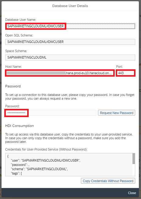
To build that view which describes the different contacts, you must create a "Database User" in the "Space Management" to access the data from Python.

I named the user DWCUSER. You have to:
- Enable the Automated Predictive Library (APL)
- Give access to the space schema's views that are exposed for consumption
- Give write access to the user's schema

When the user is created, you need the host name, the port (always 443) and the password, which is automatically created.
Start the local Python development environment of your choice. I am using Jupyter Notebooks, that were installed through Anaconda. Install the hana_ml library.
!pip install hana_mlAs a quick test, you can check the connection from your Python environment to the SAP Data Warehouse Cloud by hardcoding the logon credentials. If this code is failing, check that SAP Datawarehouse Cloud is allowing access to your IP address.
import hana_ml.dataframe as dataframe

conn = dataframe.ConnectionContext("YOURHOSTNAME",

                                   443,

                                   "YOURUSER",

                                   "YOURPASSWORD",

                                   encrypt = True,

                                   sslValidateCertificate = False)


# Send basic SELECT statement and display the result

sql = 'SELECT 12345 FROM DUMMY'

df_remote = conn.sql(sql)

print(df_remote.collect())
If the above test worked, store the password securely in the hdbuserstore application, which is part of the SAP HANA client. The Hands-On Tutorial: Machine Learning push-down to SAP HANA with Python describes this in a little more detail, but the credentials are stored with:
C:\Program Files\SAP\hdbclient>hdbuserstore -i SET DWC_SMC "YOURHOSTNAME":443 SAPMARKETINGCLOUDML#DWCUSER
The logon can then simply refer to those stored credentials.
import hana_ml.dataframe as dataframe


# Instantiate connection object

conn = dataframe.ConnectionContext(userkey="DWC_SMC",

                                   encrypt = True,

                                   sslValidateCertificate = False)


# Send basic SELECT statement and display the result

sql = 'SELECT 12345 FROM DUMMY'

df_remote = conn.sql(sql)

print(df_remote.collect())
Comment on SAP Data Intelligence: If you were using SAP Data Intelligence, the logon credentials would be saved in a connection in SAP Data Intelligence. Python would be scripted in Jupyter Notebooks within a Machine Learning Scenario. A local Python installation would not be required.
First you may want to explore the data. Take a peek at a few rows.
import pandas as pd

pd.set_option('display.max_columns', None)

df_remote_interactions = conn.table("V_I_MKT_INTERACTION", schema = "SAPMARKETINGCLOUDML")

df_remote_interactions.head(5).collect()
Or count for instance how often the different interaction types occur. Here the 10 most frequent are displayed. It's a demo system with fake data, most sent emails bounced.
df_agg = df_remote_interactions.agg([('count', 'Interaction', 'InteractionTypeCount')], group_by = 'InteractionType').collect()

df_agg.sort_values(by = 'InteractionTypeCount', ascending = False).head(10)
Now we need to build the data set for the Machine Learning model, filtered and aggregated as described at the beginning of this chapter. You can be very creative in this step, particularly in creating columns that describe the contacts' past behaviour. In this example we look at a few select activities such as web site visits and searches on the website. To make this most relevant for our business scenario (purchase in the following 30 days), we count how many of these interactions a person had in the 30 days before the reference date, how many in another 30 day period further back (so days 60 to 31 before the reference date) and how the behaviour changed between these two time periods.
Identify the contacts who had not purchased anything by the specified date and create a flag to indicate, whether they did purchase in the following 30 days. That flag will be the target of the Machine Learning model. For now we are hardcoding the 1st of September 2021. Later on we will turn this into a parameter, for which you can specify any date. We will also reduce the dataset to contain only contacts who had an interaction with us in the past 180 days.
# Distinct list of contacts who had purchased before the chosen date

df_remote_contacts_purchasedbefore = df_remote_interactions.filter(""""InteractionType" = 'SALES_ORDER' AND "InteractionTimeStampUTC" < '2021-09-01'""")

df_remote_contacts_purchasedbefore = df_remote_contacts_purchasedbefore.distinct("InteractionContact")

df_remote_contacts_purchasedbefore = df_remote_contacts_purchasedbefore.select('*', (1, 'PURCHASEDBEFORETARGETPERIOD'))


# Distinct list of contacts who had purchased in the chosen target period (30 days after the chosen date)

df_remote_purchasedintargetperiod = df_remote_interactions.filter(""""InteractionType" = 'SALES_ORDER' AND "InteractionTimeStampUTC" BETWEEN '2021-09-01' and ADD_DAYS('2021-09-01', 30)""")

df_remote_purchasedintargetperiod = df_remote_purchasedintargetperiod.distinct("InteractionContact")

df_remote_purchasedintargetperiod = df_remote_purchasedintargetperiod.select('*', (1, 'PURCHASEINTARGETPERIOD'))


#  Distinct list of all contacts who had an interaction in the 180 days before the chosen date

df_remote_contacts_all = df_remote_interactions.filter(""" "InteractionTimeStampUTC" > ADD_DAYS('2021-09-01', -180)""").distinct("InteractionContact")

#df_remote_contacts_all = df_remote_interactions.distinct("InteractionContact")


# Join and filter the dataset to obtain the population of interest, contacts who had not purchased by the chosen date

df_remote_contacts_all.set_index("InteractionContact")

df_remote_contacts_purchasedbefore.set_index("InteractionContact")

df_remote_purchasedintargetperiod.set_index("InteractionContact")

df_remote_population = df_remote_contacts_all.join([df_remote_contacts_purchasedbefore, df_remote_purchasedintargetperiod], how = 'left')

df_remote_population = df_remote_population.filter("PURCHASEDBEFORETARGETPERIOD IS NULL")
Next we need to describe these contacts, who they are and how they behaved in the time before the chosen date. You could potentially add demographic data such as gender or language from the I_MKT_CONTACT provider. However, there is a risk to introduce an unethical bias. You would have to make sure that using such information is suitable in your case. If you have decided you can use such demographic data, then enrich your contact with the following code. In this blog, we decided not to make use of any such data and the 'LanguageCode' from the following example will not be used.
df_remote_contacts = conn.table("V_I_MKT_CONTACT", schema = "SAPMARKETINGCLOUDML")

df_remote_contacts = df_remote_contacts.select(['InteractionContact', 'LanguageCode']).set_index("InteractionContact")

df_remote_population = df_remote_population.set_index("InteractionContact").join(df_remote_contacts)
In this blog, the contacts are only described through calculated columns that reflect their interactions. These columns will be used as predictors in the Machine Learning model. Create multiple sets of predictors that will be joined later on.
Our contacts' behaviour 30 days before the chosen date:
df_remote_behaviour = conn.table("V_I_MKT_INTERACTION", schema = "SAPMARKETINGCLOUDML")

df_remote_behaviour1m = df_remote_behaviour.filter(""""InteractionTimeStampUTC" BETWEEN ADD_DAYS('2021-09-01', -30) and '2021-09-01'""")

df_remote_population_agg_1m = df_remote_population.select(['InteractionContact']).set_index("InteractionContact").join([

    df_remote_behaviour1m.filter(""""InteractionType" = 'WEBSITE_SEARCH'""").agg([("count", "InteractionType", "WEBSITE_SEARCH_1M_COUNT")], group_by = 'InteractionContact').set_index("InteractionContact"),

    df_remote_behaviour1m.filter(""""InteractionType" = 'WEBSITE_VISIT'""").agg([("count", "InteractionType", "WEBSITE_VISIT_1M_COUNT")], group_by = 'InteractionContact').set_index("InteractionContact"),

    df_remote_behaviour1m.filter(""""InteractionType" = 'WEBSITE_VIDEO'""").agg([("count", "InteractionType", "WEBSITE_VIDEO_1M_COUNT")], group_by = 'InteractionContact').set_index("InteractionContact"),

    df_remote_behaviour1m.filter(""""InteractionType" = 'WEBSITE_DOWNLOAD'""").agg([("count", "InteractionType", "WEBSITE_DOWNLOAD_1M_COUNT")], group_by = 'InteractionContact').set_index("InteractionContact"),

    df_remote_behaviour1m.filter(""""InteractionType" = 'SHOP_ITEM_VIEW'""").agg([("count", "InteractionType", "SHOP_ITEM_VIEW_1M_COUNT")], group_by = 'InteractionContact').set_index("InteractionContact"),

    df_remote_behaviour1m.filter(""""InteractionType" = 'EMAIL_OPENED'""").agg([("count", "InteractionType", "EMAIL_OPENED_1M_COUNT")], group_by = 'InteractionContact').set_index("InteractionContact")

], how = 'left')
Their behaviour in the 30 days further back in the past:
df_remote_behaviour2m = df_remote_behaviour.filter(""""InteractionTimeStampUTC" BETWEEN ADD_DAYS('2021-09-01', -60) and ADD_DAYS('2021-09-01', -30)""")

df_remote_population_agg_2m = df_remote_population.select(['InteractionContact']).set_index("InteractionContact").join([

    df_remote_behaviour2m.filter(""""InteractionType" = 'WEBSITE_SEARCH'""").agg([("count", "InteractionType", "WEBSITE_SEARCH_2M_COUNT")], group_by = 'InteractionContact').set_index("InteractionContact"),

    df_remote_behaviour2m.filter(""""InteractionType" = 'WEBSITE_VISIT'""").agg([("count", "InteractionType", "WEBSITE_VISIT_2M_COUNT")], group_by = 'InteractionContact').set_index("InteractionContact"),

    df_remote_behaviour2m.filter(""""InteractionType" = 'WEBSITE_VIDEO'""").agg([("count", "InteractionType", "WEBSITE_VIDEO_2M_COUNT")], group_by = 'InteractionContact').set_index("InteractionContact"),

    df_remote_behaviour2m.filter(""""InteractionType" = 'WEBSITE_DOWNLOAD'""").agg([("count", "InteractionType", "WEBSITE_DOWNLOAD_2M_COUNT")], group_by = 'InteractionContact').set_index("InteractionContact"),

    df_remote_behaviour2m.filter(""""InteractionType" = 'SHOP_ITEM_VIEW'""").agg([("count", "InteractionType", "SHOP_ITEM_VIEW_2M_COUNT")], group_by = 'InteractionContact').set_index("InteractionContact"),

    df_remote_behaviour2m.filter(""""InteractionType" = 'EMAIL_OPENED'""").agg([("count", "InteractionType", "EMAIL_OPENED_2M_COUNT")], group_by = 'InteractionContact').set_index("InteractionContact")

], how = 'left')
Join the columns of those two subsequent 30 day periods:
df_remote_population.set_index("InteractionContact")

df_remote_population_agg_1m.set_index("InteractionContact")

df_remote_population_agg_2m.set_index("InteractionContact")

df_remote_population_360 = df_remote_population.join([df_remote_population_agg_1m, df_remote_population_agg_2m], how = 'left')
Many of these columns show null values. If a person didn't visit the website, there is nothing to count and the result is a null value. Change those null values to numerical zeros.
numeric_columns = []

for column_name in df_remote_population_360.columns:

    if df_remote_population_360.is_numeric(column_name):

        numeric_columns.append(column_name)

df_remote_population_360 = df_remote_population_360.fillna(0, numeric_columns)
Calculate further information, how the behaviour changed between those two periods. If a person becomes more active on your website for instance, this could be a good indicator for the intend to purchase a product.
df_remote_population_360 = df_remote_population_360.select('*',

                                                           ('WEBSITE_SEARCH_1M_COUNT - WEBSITE_SEARCH_2M_COUNT', 'WEBSITE_SEARCH_COUNT_DELTA'),

                                                           ('WEBSITE_VISIT_1M_COUNT - WEBSITE_VISIT_2M_COUNT', 'WEBSITE_VISIT_COUNT_DELTA'),

                                                           ('WEBSITE_VIDEO_1M_COUNT - WEBSITE_VIDEO_2M_COUNT', 'WEBSITE_VIDEO_COUNT_DELTA'),

                                                           ('WEBSITE_DOWNLOAD_1M_COUNT - WEBSITE_DOWNLOAD_2M_COUNT', 'WEBSITE_DOWNLOAD_COUNT_DELTA'),

                                                           ('SHOP_ITEM_VIEW_1M_COUNT - SHOP_ITEM_VIEW_2M_COUNT', 'SHOP_ITEM_VIEW_DELTA'),

                                                           ('EMAIL_OPENED_1M_COUNT - EMAIL_OPENED_2M_COUNT', 'EMAIL_OPENED_DELTA'),

                                                           )
Carry out some tidy ups.
# Drop the column that was created for the filtering on customers that had never purchased before

df_remote_population_360 = df_remote_population_360.drop("PURCHASEDBEFORETARGETPERIOD")


# Cast all numerical columns to INT, which will help later on as that format allows more data exploration

numeric_columns = []

for column_name in df_remote_population_360.columns:

    if df_remote_population_360.is_numeric(column_name):

        numeric_columns.append(column_name)

df_remote_population_360 = df_remote_population_360.cast(numeric_columns, 'INT')


# Cast the target variable to NVARCHAR. This is needed for the clasification Machine Learning model

df_remote_population_360 = df_remote_population_360.cast('PURCHASEINTARGETPERIOD', 'NVARCHAR(10)')
Have a look at the contents of the columns. Depending on your data volume, this could take a few minutes.
df_remote_population_360.describe().collect()
We have the customer view, but we want this parameterised, so that you can easily specify the date around which the logic builds up. Use the SELECT statement that the hana_ml library created for the above view, to create the SQL syntax that creates a parameterised view. The hardcoded date of 1 September 2021 becomes a parameter called P_REFERENCEDATE.
reference_date = '2021-09-01'

sql_createview = df_remote_population_360.select_statement

sql_createview = sql_createview.replace("'" + reference_date + "'", ":P_REFERENCEDATE")

sql_createview = "CREATE  VIEW VP_FIRSTPURCHASEIN30DAYS(IN P_REFERENCEDATE NVARCHAR(10)) AS " + sql_createview + ";"
Execute the SQL code and you have the view, which can be used both for training the model and applying the model by passing different reference dates as parameter.
from hdbcli import dbapi

dbapi_cursor = conn.connection.cursor()

dbapi_cursor.execute(sql_createview)
As a quick test, call the view with a different reference date and look at a few rows.
df_remote_population_360 = conn.sql("SELECT * FROM VP_FIRSTPURCHASEIN30DAYS('2021-08-15')")

df_remote_population_360.sort("WEBSITE_SEARCH_1M_COUNT", desc = True).head(5).collect()
Machine Learning Training and Prediction
We are good to use the Machine Learning now! Create a pointer to the new view, with the reference date for training the model.
df_remote_train = conn.sql("SELECT * FROM VP_FIRSTPURCHASEIN30DAYS('2021-09-01')").sort("InteractionContact", desc = False)Have the hana_ml library create a report on the dataset to explore the structure and content of the data. There are many other options to explore the data with hana_ml, always pushing down any calculation to SAP Data Warehouse Cloud. it might take a minute for this report to show up.
from hana_ml.visualizers.unified_report import UnifiedReport

UnifiedReport(df_remote_train).build().display()
Configure and train the Machine Learning model. Here we work with the standard configuration of the Automated Predictive Library. You have many options to configure this process, see for instance the documentation of the GradientBoostingClassifier.
from hana_ml.algorithms.apl.gradient_boosting_classification import GradientBoostingBinaryClassifier

col_target = 'PURCHASEINTARGETPERIOD' # Targe column

target_value = '1' # The behaviour the model will predict

col_id = 'InteractionContact' # ID column

gbapl_model = GradientBoostingBinaryClassifier()

gbapl_model.set_params(target_key = target_value) # The behaviour the model will predict

gbapl_model.fit(data = df_remote_train,

                key = col_id,

                label = col_target)
You can interpret the trained model's logic. This is often referred to as Global Explainable AI). There is another standard report to look at the Machine Learning model.
from hana_ml.visualizers.unified_report import UnifiedReport

%matplotlib auto

UnifiedReport(gbapl_model).build().display()

%matplotlib inline
The Area Under the Curve (AUC) is a fantastic 0.961. We are working with demo data. On your own real, productive data please don't expect such a strong model. The three most important columns for the prediction of who will make their first purchase in the next 30 days are:
- WEBSITE_SEARCH_COUNT_DELTA - Change between the two periods in how often the contact searched on the website
- WEBSITE_DOWNLOAD_1M_COUNT - How often the contact downloaded material in the most recent 30 days
- WEBSITE_VISIT_1M_COUNT - How often the contact visited the website in the most recent 30 days
The trained Model can be interpreted deeper than what is exposed in the report above. So far we know that WEBSITE_SEARCH_COUNT_DELTA is very important. But what are the values that correspond with a higher or lower probability of the contact making their first purchase?
variable_name = 'WEBSITE_SEARCH_COUNT_DELTA'


import seaborn as sns

import matplotlib.pyplot as plt

df_category_signif = gbapl_model.get_indicators().filter("KEY = 'GroupSignificance' and VARIABLE = '" + variable_name + "'").collect()

df_category_signif = df_category_signif[['VARIABLE', 'TARGET', 'DETAIL', 'VALUE']]

df_category_signif['VALUE'] = df_category_signif['VALUE'].astype(float).round(2)

df_category_signif.columns = ['Predictor', 'Target','Category','Significance']

df_category_signif = df_category_signif.sort_values(by = ['Significance'], ascending = False)

plt.figure()

bplot = sns.barplot(data = df_category_signif, x = 'Category', y = 'Significance', color = '#1f77b4')

bplot.set_title(variable_name)

bplot.set_xticklabels(bplot.get_xticklabels(), rotation = 45);
Contacts who searched 6-times more often in the most recent 30 days than in the 30 days further back have the highest probability of their first purchase. Contacts who searched 1 to 5 times more often still have an increased probability.
We looked at the Machine Learning model, we are happy with it, so let's predict. Use the view with the reference date of today (we pretend it is 1 October 2021) to predict the probability of a first purchase in the next 30 days.
df_remote_apply = conn.sql("SELECT * FROM VP_FIRSTPURCHASEIN30DAYS('2021-10-01')")

df_remote_apply = df_remote_apply.drop("PURCHASEINTARGETPERIOD")

gbapl_model.set_params(extra_applyout_settings =

                        {'APL/ApplyExtraMode': 'Advanced Apply Settings',

                         'APL/ApplyDecision': 'true',

                         'APL/ApplyProbability': 'true',

                         'APL/ApplyPredictedValue': 'true'

                        })

df_remote_predict = gbapl_model.predict(df_remote_apply)
Look at the predictions. The column gb_proba_PURCHASEINTARGETPERIOD is the probability that is relevant for us. The column gb_score_PURCHASETARGETPERIOD is an intermediate value, which is not required for us.
df_remote_predict.head(5).collect()
Save the predictions to a table, from where they can be sent to SAP Marketing Cloud.
df_remote_predict.save("PRED_FIRSTPURCHASEIN30DAYS" , force = True)Machine Learning Operations and Reporting (optional)
Over time your model should be retrained regularly. You may (or may not) want to have a dashboard to track the different models. Every time a new model gets trained you can store any relevant information in a table in SAP Data Warehouse Cloud and report off it with SAP Analytics Cloud.
Collect the values you want to store. As usual, this is an example, you may care about very different pieces of information that you want to report on.
import pandas as pd

mlrepo_dateime = pd.Timestamp.now()

mlrepo_modelname = 'New customer will purchase in next 30 days'

mlrepo_traincount = df_remote_train.count()

mlrepo_positivecount = df_remote_train.filter(col_target +' = ' + target_value).count()

mlrepo_auc = gbapl_model.get_performance_metrics()['AUC']
Bring these values into a pandas DataFrame and upload it to SAP Data Warehouse Cloud.
# Create pandas DataFrame

data = {'MODELDATETIME': [mlrepo_dateime],

        'MODELNAME': [mlrepo_modelname],

        'TRAINCOUNT': [mlrepo_traincount],

        'POSITIVECOUNT': [mlrepo_positivecount],

        'AUC': [mlrepo_auc]}

df_data = pd.DataFrame(data)

df_data.MODELDATETIME = pd.to_datetime(df_data.MODELDATETIME)


# Upload to SAP Data Warehouse Cloud

df_remote = dataframe.create_dataframe_from_pandas(connection_context = conn,

                                                   pandas_df = df_data,

                                                   table_name = 'MLREPO',

                                                   drop_exist_tab = False,

                                                   force = False,

                                                   replace = False)
The ML operations data is stored in SAP Data Warehouse Cloud. Expose the data as a view with "Semantic Usage" set to "Analytical Dataset", expose it for consumption and run it in "Analytical Mode".
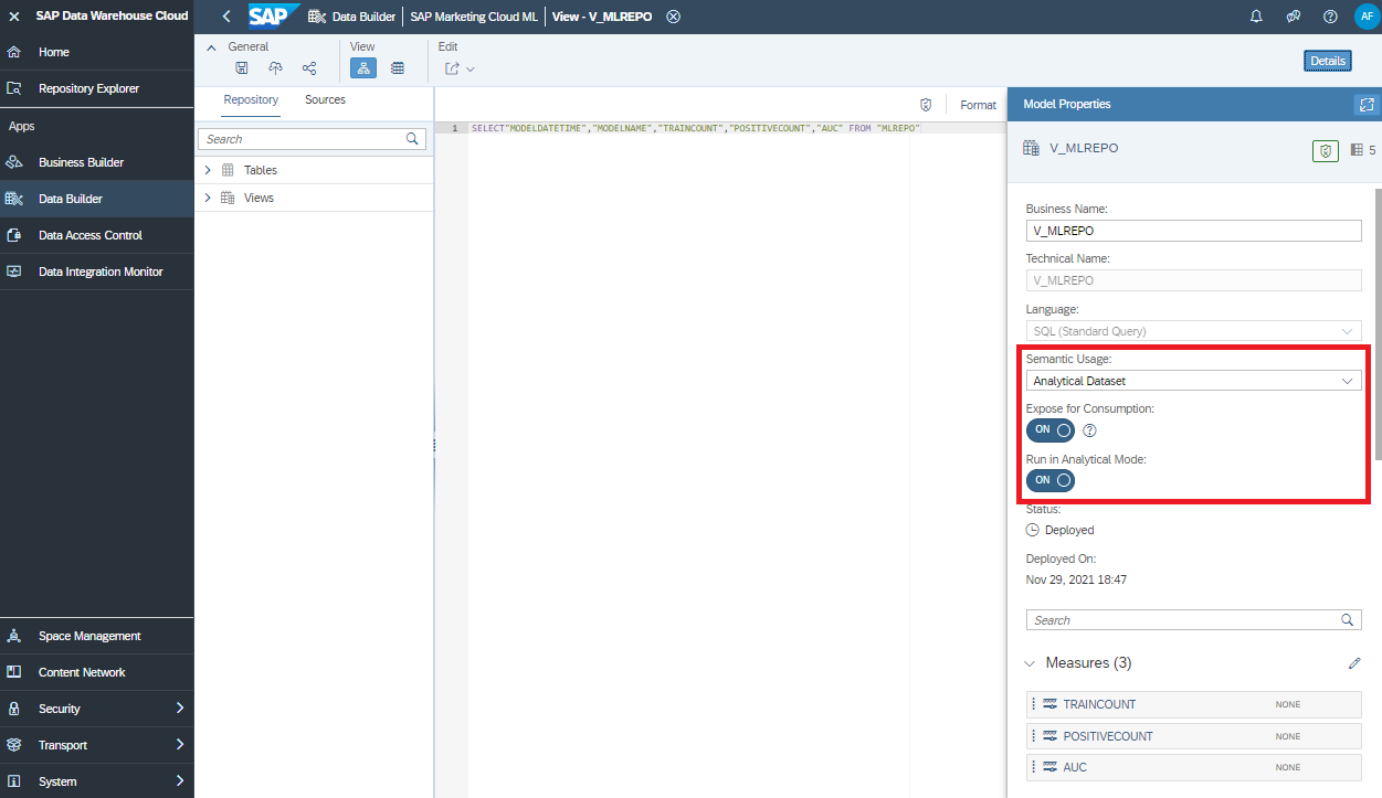
In SAP Analytics Cloud connect to that view with a live connection...

... and create a dashboard that fits your requirements!

Passing the Predictive Scores to SAP Marketing Cloud
The predictive scores are in a table in SAP HANA. Now pass them to the SAP Marketing Cloud through the Score API. Please also see the blog "Use the Marketing Score API to push externally calculated Score Values to SAP Marketing Cloud" that explains how to configure SAP Marketing Cloud to receive the predictions.
You can use any tool of your choice to upload the data. We stick with Python, as this will allow us to schedule all steps (ML training, prediction, upload) in one program.
Before uploading all scores, let's have a look at an example. You need the credentials for SAP Marketing Cloud. This could be the same user that was used for the real time replication.
smc_system = 'https://YOURSMC-api.s4hana.ondemand.com/' # Make sure to use the -api

smc_api_user = 'YOURTECHNICALSMCUSER'

smc_api_pwd = 'YOURTECHNICALSMCPASSWORD'
The first call to the REST-API obtains a csrf token.
import requests

s = requests.Session()

s.headers.update({'Connection': 'keep-alive'})


url = smc_system + "sap/opu/odata/sap/API_MKT_SCORE_SRV/"


headers = {

  'x-csrf-token': 'fetch'

}


response = requests.request("GET", url, headers = headers, auth = (smc_api_user, smc_api_pwd))

my_csrf_token = response.headers['x-csrf-token']
Collect the retrieved cookies.
col = []

my_csrf_cookies = response.cookies.get_dict()

for key, value in my_csrf_cookies.items():

        col.append(key + "=" + value)

my_csrf_cookies_concat = '; '.join(col)
With the csrf token and the cookies you can upload scores to SAP Marketing Cloud. A few things to note here:
- In the example 'YY1_BUYINGPROBABILITYSCORE' is the name of the scenario created in SAP Marketing Cloud. You must change this to the name of your scenario.
- Similarly, change the value of the 'MarketingScoreModel' to the value of your own.
- The scores are associated with a time stamp that has to be in UTC time.
- The 'MarketingScoredObjectUUID' is the hyphened InteractionContact.
- The 'MarketingScoreValue' is the predicted probability, which has to be passed as string.
import requests

import json


url = smc_system + "sap/opu/odata/sap/API_MKT_SCORE_SRV/Scores(MarketingScore='YY1_BUYINGPROBABILITYSCORE')/ScoreModels"


payload = json.dumps({

  "MarketingScore": "YY1_BUYINGPROBABILITYSCORE",

  "MarketingScoreModel": "0000000372",

  "ScoreValues": [

    {

      "MarketingScoreDateTime": "2021-10-01T15:00:00",

      "MarketingScoredObjectUUID": "FA163EA9-0DDA-1EEB-BFFC-10635C0E922D",

      "MarketingScoreValue": "0.032824"

    },

    {

      "MarketingScoreDateTime": "2021-10-01T15:00:00",

      "MarketingScoredObjectUUID": "FA163EA9-0DDA-1EDC-889C-2EC843DBCCDE",

      "MarketingScoreValue": "0.733358"

    }

  ]

})

headers = {

  'x-csrf-token': my_csrf_token,

  'Cookie': my_csrf_cookies_concat,

  'Content-Type': 'application/json'

}


response = requests.request("POST", url, headers=headers, data=payload, auth = (smc_api_user, smc_api_pwd))
The call returns its response in XML format.
from bs4 import BeautifulSoup

bs = BeautifulSoup(response.text)

pretty_xml = bs.prettify()

print(pretty_xml)
If the upload was successful, the first few lines should look like the above. The full response is longer. If the upload ran into an error, the response will start with an error message.
And now with the real predictions, that are saved in SAP HANA. An informal suggestion of a colleague is to upload up to 250 thousand scores with a single REST-API call. The dataset in this example is smaller, so a single upload of all data at once should work. But to show the concept, of breaking the data down into smaller segments, the example below is uploading the data in batches of just 10 thousand.
# Logon to SAP HANA Cloud
import hana_ml.dataframe as dataframe
conn = dataframe.ConnectionContext(userkey="DWC_SMC",
encrypt = True,
sslValidateCertificate = False)
# Point to the table that contains the predictions
df_remote_predict = conn.table("PRED_FIRSTPURCHASEIN30DAYS")
# New column that hyphens the InteractionContact
df_remote_predict = df_remote_predict.select('*', ('''Left("InteractionContact", 😎 || '-' ||
Substring("InteractionContact", 9, 4) || '-' ||
Substring("InteractionContact", 13, 4) || '-' ||
Substring("InteractionContact", 17, 4) || '-' ||
Right("InteractionContact", 12)''', "MARKETINGSCOREOBJECTUUID"))
# Add the MarketingScoreDateTime
import datetime
str_datetime = datetime.datetime.now(datetime.timezone.utc).isoformat()
df_remote_predict = df_remote_predict.select('*', (''' '{0}' '''.format(str_datetime), 'MarketingScoreDateTime'))
# Select and rename the three relevant columns MarketingScoreDateTime, MarketingScoredObjectUUID, MarketingScoreValue
df_remote_predict = df_remote_predict.select("MarketingScoreDateTime", ("MARKETINGSCOREOBJECTUUID", "MarketingScoredObjectUUID"), ('"gb_proba_PURCHASEINTARGETPERIOD"', "MarketingScoreValue"))
# For the REST-API call
url = smc_system + "sap/opu/odata/sap/API_MKT_SCORE_SRV/Scores(MarketingScore='YY1_BUYINGPROBABILITYSCORE')/ScoreModels"
headers = {
'x-csrf-token': my_csrf_token,
'Cookie': my_csrf_cookies_concat,
'Content-Type': 'application/json'
}
# Add a bin column that allows to split the data into multiple smaller uploads
batchsize = 10000
df_remote_predict = df_remote_predict.add_id()
import math
for ii in range(math.ceil(df_remote_predict.count() / batchsize)):
# Format the data that is to be uploaded
df_remote_toupload = df_remote_predict.filter("ID > " + str(ii * batchsize) + " AND ID <= " + str((ii + 1) * batchsize))
df_toupload = df_remote_toupload.drop("ID").collect()
df_toupload['MarketingScoreValue'] = df_toupload['MarketingScoreValue'].round(4)
df_toupload['MarketingScoreValue'] = df_toupload['MarketingScoreValue'].astype(str)
# Upload the data
import requests, json
dict_toupload = df_toupload.to_dict(orient = 'records')
payload = json.dumps({
'MarketingScore': "YY1_BUYINGPROBABILITYSCORE",
"MarketingScoreModel": "0000000372",
"ScoreValues": dict_toupload
})
response = requests.request("POST", url, headers=headers, data=payload, auth = (smc_api_user, smc_api_pwd))
# Print status update
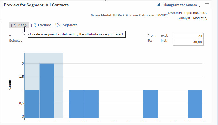
print("Segment " + str(ii) + " done, count: " + str(df_toupload.shape[0]))The predictions are available in SAP Marketing Cloud, ready for use in your campaigns!
Scheduling (optional)
If you need updated predictions in SAP Marketing Cloud only once in a while, you might be happy to manually run the Python code, and your implementation is complete. Most likely the predictions need to be kept up to date much more frequently though, hence scheduling the above logic is required.
You can bring all relevant code (training, applying, uploading) into a Python file, that can be scheduled any way you like. Maybe you already have a server on which to deploy that schedule. The code of that file became too large to be posted here. If you are interested in it just send me a message and I will email it.
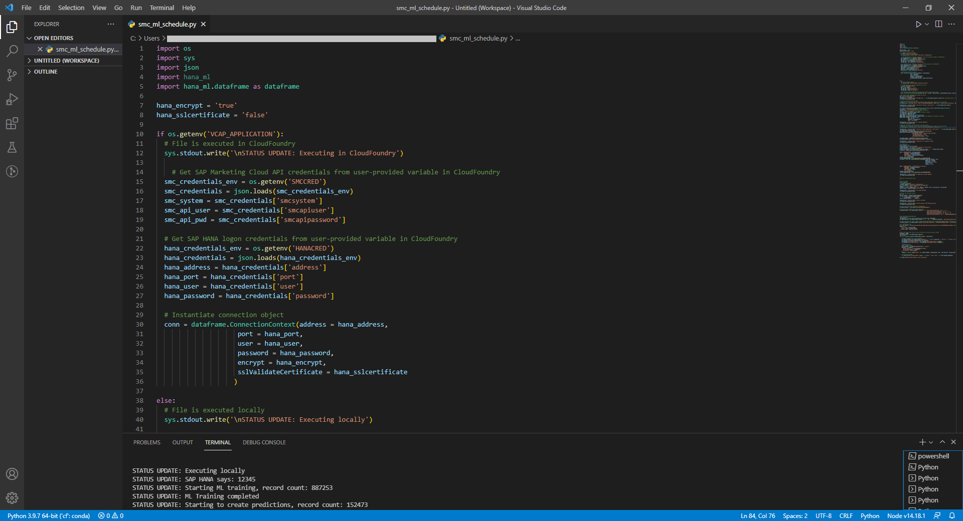
However, you can also rely on the SAP Business Technology Platform to host and schedule the code. That Python file can be deployed on a Cloud Foundry environment, and scheduled with the BTP's Job Scheduling Service. An example of scheduling Python code that uses the hana_ml wrapper is in the blog Scheduling Python code on Cloud Foundry.

Comment on SAP Data Intelligence: If you have SAP Data Intelligence you would use it's scheduling capabilities, there would be no need for Cloud Foundry.
Summary
And you are done! You have extended SAP Marketing Cloud with the SAP Business Technology Platform to improve your campaigns through Machine Learning.
- The Marketeer benefits from the latest predictions in their campaigns, without having to be a Data Scientist
- The Data Scientist has full control and visibility into the Machine Learning
- The IT department is in charge of the deployment
The circle has been closed!
But the story can continue. With the Machine Learning algorithms in the SAP Data Warehouse Cloud you can implement many other scenarios. You may want to create other predictions for use in SAP Marketing Cloud. But very different scenarios are also possible. Just one example: A Kaplan-Meier analysis of the customer lifetime can provide a lot of insight you may want to consider in your campaigns to reduce the churn risk.

Happy predicting!
Labels:
11 Comments
You must be a registered user to add a comment. If you've already registered, sign in. Otherwise, register and sign in.
Labels in this area
-
ABAP CDS Views - CDC (Change Data Capture)
2 -
AI
1 -
Analyze Workload Data
1 -
BTP
1 -
Business and IT Integration
2 -
Business application stu
1 -
Business Technology Platform
1 -
Business Trends
1,658 -
Business Trends
110 -
CAP
1 -
cf
1 -
Cloud Foundry
1 -
Confluent
1 -
Customer COE Basics and Fundamentals
1 -
Customer COE Latest and Greatest
3 -
Customer Data Browser app
1 -
Data Analysis Tool
1 -
data migration
1 -
data transfer
1 -
Datasphere
2 -
Event Information
1,400 -
Event Information
74 -
Expert
1 -
Expert Insights
177 -
Expert Insights
348 -
General
1 -
Google cloud
1 -
Google Next'24
1 -
GraphQL
1 -
Kafka
1 -
Life at SAP
780 -
Life at SAP
14 -
Migrate your Data App
1 -
MTA
1 -
Network Performance Analysis
1 -
NodeJS
1 -
PDF
1 -
POC
1 -
Product Updates
4,575 -
Product Updates
391 -
Replication Flow
1 -
REST API
1 -
RisewithSAP
1 -
SAP BTP
1 -
SAP BTP Cloud Foundry
1 -
SAP Cloud ALM
1 -
SAP Cloud Application Programming Model
1 -
SAP Datasphere
2 -
SAP S4HANA Cloud
1 -
SAP S4HANA Migration Cockpit
1 -
Technology Updates
6,871 -
Technology Updates
482 -
Workload Fluctuations
1
Related Content
- Your Ultimate Guide for SAP Sapphire 2024 Orlando in Technology Blogs by SAP
- Technovation Summit 2024: Expand your AI and BTP Horizons in Technology Blogs by SAP
- End-to-end Processes and modular processes in SAP Signavio Process Insights, discovery edition in Technology Blogs by SAP
- Understanding Data Modeling Tools in SAP in Technology Blogs by SAP
- IoT - Ultimate Data Cyber Security - with Enterprise Blockchain and SAP BTP 🚀 in Technology Blogs by Members
Top kudoed authors
| User | Count |
|---|---|
| 15 | |
| 11 | |
| 10 | |
| 10 | |
| 9 | |
| 8 | |
| 7 | |
| 7 | |
| 7 | |
| 7 |