
- SAP Community
- Products and Technology
- Technology
- Technology Blogs by SAP
- Anomaly Detection in Time-Series using Seasonal De...
Technology Blogs by SAP
Learn how to extend and personalize SAP applications. Follow the SAP technology blog for insights into SAP BTP, ABAP, SAP Analytics Cloud, SAP HANA, and more.
Turn on suggestions
Auto-suggest helps you quickly narrow down your search results by suggesting possible matches as you type.
Showing results for
Advisor
Options
- Subscribe to RSS Feed
- Mark as New
- Mark as Read
- Bookmark
- Subscribe
- Printer Friendly Page
- Report Inappropriate Content
12-21-2020
7:58 AM
A time-series is a collection of data points/values ordered by time, often with evenly spaced time-stamps. For example, an air-quality monitoring system continuously measures the air quality around it, and sends out the air-quality-index(AQI) values so we get the time-series of AQIs. In this case, malfunction of the monitoring system or unexpected local incidents(like fire-accident) can bring sudden changes of AQIs temporarily, causing the obtained values to appear anomalous. Sometimes the detection of anomalous points in a time-series could be as simple as statistical tests, yet frequently the task will be much more difficult since there is no guarantee that the anomalous points are directly associated with extreme values. However, statistical tests for anomaly/outlier detection could become applicable to the time-series data if appropriate modeling is applied.
In this blog post, we will focus on the detection of anomalies/outliers in time-series that can be largely explained by a smoothing trend together with a single seasonal pattern. Such time-series usually can be modeled well enough by seasonal-trend decomposition, or seasonal decomposition for simplicity. The seasonal decomposition method is provided in SAP HANA Predictive Analysis Library(PAL), and wrapped up in the Python Machine Learning Client for SAP HANA(hana_ml) . Basically, in this blog post you will learn:
- How to apply seasonal decomposition to the time-series data of interest and interpreting the statistics w.r.t. the decomposition.
- How detection of anomalies/outliers is done after seasonal decomposition is applied to the time-series data.
Introduction
The detection of anomalies from a given time-series is usually not an easy task. The natural association with time brings many unique features to time-series that regular 1D datasets, like time-dependency(via lagging), trend, seasonality, holiday effects, etc. Because of this, traditional statistical tests or clustering-based methods for anomaly/outlier usually will fail for time-series data, because the time information of time-series is ignored by their design of nature. In other words, the applicability of statistical tests at least requires time-series data values to be time-independent, yet this is often not guaranteed. However, with appropriated modeling, a roughly time-independent time-series can often be extracted/transformed from the original time-series of interest, in which case statistical tests becomes applicable. One such technique, also the main interest of this blog post, is seasonal decomposition.
Basically, seasonal decomposition decomposes a given time-series into three components: trend, seasonal and random, where:
- the seasonal component contains patterns that appears repeatedly between regular time-intervals(i.e. periods)
- the trend component depicts the global shape of the time-series by smoothing/averaging out local variations/seasonal patterns
- the random component contains information that cannot be explained by seasonal and trend components(values assumed to be random, indicating time-independent)
The relation between the original time-series data and its decomposed components in seasonal decomposition can either be additive or multiplicative. To be formal, we let X be the given time-series, and S/T/R be its seasonal/trend/random component respectively, then
- multiplicative decomposition: X = S * T * R
- additive decomposition: X = S + T + R
It should be emphasized that, for multiplicative decomposition, values in the random component are usually centered around 1, where the value of 1 means that the original time-series can be perfectly explained by the multiplication of its trend and seasonal components. In contrast, for additive decomposition, values in the random component are usually centered around 0, where the value of 0 indicates that the given time-series can be perfectly explained by the addition of its trend and and seasonal components.
In this blog post, we focus on anomaly detection for time-series that can largely be modeled by seasonal decomposition. In such case, anomalous points are marked by values with irregularly large deviations in the random component, which correspond to unexplained large variations beyond trend and seasonality.
The Use Case : Anomaly Detection for AirPassengers Data
In the following context we show a detailed use case for anomaly detection of time-series using seasonal decomposition, and all source code will use use Python machine learning client for SAP HANA Predictive Analysis Library(PAL). The dataset we use is the renowned AirPassengers dataset firstly introduced in a textbook for time-series analysis written by Box and Jenkins.
Connection to SAP HANA
Assuming the dataset is stored in SAP HANA as a table with name 'AIR_PASSENGERS_TBL'. Then, we can fetch the data via a connection to the database.
import hana_ml

from hana_ml.dataframe import ConnectionContext

cc = ConnectionContext('xx.xxx.xxx.xx', 30x15, 'XXX', 'Xxxxxxxx')#account info hidden away

ap_tbl_name = 'AIR_PASSENGERS_TBL'

ap_df = cc.table(ap_tbl_name)
Dataset Description and Pre-processing
The AirPassengers dataset is a monthly record of total airline passengers between 1949 and 1960, illustrated as follows:
ap_data = ap_df.collect()

ap_data

The dataset contains two columns : the first column is the month info(represented by the first day of each month), and the second column is the number of passengers(in thousands). Now we draw the run-sequence plot of this dataset for better inspecting its shape and details.
import matplotlib.pyplot as plt

plt.plot(pd.to_datetime(ap_data['Month']), ap_data['#Passengers'])

plt.show()

Before applying any time-series analysis method to this dataset, we add an ID column of integer type. We do so because an ID column of integer type is a must for most time-series algorithms in hana_ml, inclusive of seasonal decomposition. Besides, the added integer ID column must represent the order of values for the time-series data, so generated IDs must follow the order of timestamps of the time-series. We can generate such an ID column using the add_id() function of hana_ml.DataFrame as follows:
ap_df_wid = ap_df.cast('Month', 'DATE').add_id(id_col='ID', ref_col='Month')Now we may check whether everything is okay after the new integer ID column has been added.
ap_df_wid.collect()

Multiplicative Decomposition
Observing from its run-sequence plot, the AirPassengers dataset clearly has trend and seasonality: the number of airline passengers keep growing year-by-year, forming an upward trend; within each year there is a clear seasonal pattern - high in year middle and low in year start/end. Note that the seasonal variations become larger as the number of passengers increases, which is a clear evidence for multiplicative seasonality. Seasonal decomposition is implemented by the function seasonal_decompose() in hana_ml, we can import the function and then apply it to the original time-series to verify our justification on the type of decomposition.
The seasonal decomposition algorithm in hana_ml does two things sequentially: firstly it tests whether the input time-series data contains any significant additive/multiplicative seasonal pattern, then it will decompose the time-series accordingly based on the seasonality test result. The returned result is a tuple of two hana_ml.DataFrames, with seasonality test result summarized in the first hana_ml.DataFrame and decomposition result in the second one.
from hana_ml.algorithms.pal.tsa.seasonal_decompose import seasonal_decompose

stat, decomposed = seasonal_decompose(data = ap_df_wid,

                                      key = 'ID',

                                      endog = '#Passengers',

                                      extrapolation=True)
The seasonal decomposition algorithm in hana_ml does two things sequentially: firstly it tests whether the input time-series data contains any significant additive/multiplicative seasonal pattern, then it will decompose the time-series accordingly based on the seasonality test result. The returned result is a tuple of two hana_ml.DataFrames, with seasonality test result summarized in the first hana_ml.DataFrame and decomposition result in the second one.
Therefore, the seasonality test result for the AirPassengers dataset can be viewed by:
stat.collect()

The result shows that a strong(with autocorrelation ~ 0.89) multiplicative yearly seasonality has been detected.
The corresponding decomposition result is illustrated as follows:
decomposed.collect()

Values in the random components are all around 1, as expected.
In the following we apply the renowned variance test to the random component for anomaly detection(where the multiplier 3 is heuristically determined from the well-known 3𝜎-rule for Gaussian random data, can be changed to other positive values).
from hana_ml.algorithms.pal.preprocessing import variance_test

test_res, _ = variance_test(data=decomposed,

                            key='ID',

                            data_col='RANDOM',

                            sigma_num=3)
In the anomaly detection result(i.e. the hana_ml.DataFrame test_res), anomalies are valued by 1 in its 'IS_OUT_OF_RANGE' column. Detailed info of the detected anomalies from the origin data can be obtained as follows:
anomalies_vt_id = cc.sql('SELECT ID FROM ({}) WHERE IS_OUT_OF_RANGE = 1'.format(test_res.select_statement))

anomalies_vt = cc.sql('SELECT * FROM ({}) WHERE ID IN ({})'.format(ap_df_wid.select_statement,

                                                                   anomalies_vt_id.select_statement))

anomalies_vt.collect()
So a single anomaly with ID 2(corresponding to February 1949) has been detected. However, there is some concern with this single anomaly point:
- firstly, the point is very close the starting time-limit, whose validity could be affected by extrapolations(required by the internal mechanism of the decomposition);
- secondly, the detected anomaly falls into the early stage of the time-series during which local level is still low, where multiplicative decomposition could be over-sensitive.
Another frequently used technique for anomaly detection is inter-quartile range(IQR) test, which is considered to be more robust to extreme anomalies. In the following we apply IQR test(with default multiplier, i.e. 1.5) to the random component of the decomposition result to see what should happen.
from hana_ml.algorithms.pal.stats import iqr

test_res, _ = iqr(data=decomposed, key='ID', col='RANDOM')

So, the anomaly point detected by variance test still remains in the IQR test result, along with the introduction of 10 newly detected anomalies. Let us inspect the corresponding residuals(i.e. random values) of these detected anomalies to determine how anomalous they are.
c.sql('SELECT * FROM ({}) WHERE ID IN (SELECT ID FROM ({}))'.format(decomposed[['ID', 'RANDOM']].select_statement, anomalies_iqr.select_statement)).collect()
A noticeable newly detected anomaly is the one with ID 135(corresponding to March 1960), which deviates the most from 1 among all newly detected anomalies. Besides, it is in a time position where level values are high, and not that close to either time-limit of the given time-series as the point with ID 2.
Now let us visualize all detected anomalies in the random component under IQR test.
import matplotlib.pyplot as plt

import numpy as np

dc = decomposed.collect()

plt.plot(ap_data['Month'], dc['RANDOM'], 'k.-')

oidx = np.array(anomalies_iqr.collect()['ID']) - 1

plt.plot(ap_data['Month'][oidx], dc.iloc[oidx, 3], 'ro')

plt.show()

Detected anomalies can also be visualized from the original time-series, illustrated as follows:
import matplotlib.pyplot as plt

import numpy as np

ap_dc = ap_df.collect()

oidx = np.array(anomalies_iqr.collect()['ID']) - 1

plt.plot(ap_dc['Month'], ap_dc['#Passengers'], 'k.-')

plt.plot(ap_dc['Month'][oidx], ap_dc['#Passengers'][oidx], 'ro')

plt.show()

If knowing roughly how many anomalies are there in the dataset, then we can select only a specified number of data points with most deviant values(w.r.t. 1 for multiplicative seasonal decomposition) in the residual component. For example. if we expect that the number of anomalies in the dataset is 2, then can use the following line of code to select them out.
top2_anomalies = cc.sql('SELECT TOP 2 ID, RANDOM FROM ({}) ORDER BY ABS(RANDOM-1) DESC'.format(decomposed.select_statement))

top2_anomalies.collect()
Visualization of the two points in the original dataset is also not difficult, with Python source code illustrated as follows:
import matplotlib.pyplot as plt

oidx = np.array(top2_anomalies.collect()['ID']) - 1

plt.plot(ap_dc['Month'], ap_dc['#Passengers'], 'k.-')

plt.plot(ap_dc['Month'][oidx], ap_dc['#Passengers'][oidx], 'ro')

plt.show()

We see that the point with ID 135 still remains, and it is not likely to be a result of boundary extrapolation, so it may worth more investigation.
In the following section we try to decompose the AirPassengers dataset using additive seasonal decomposition model.
Additive Decomposition
As is known to all, a multiplicative model can be transformed to an additive one by taking logarithm transformation. So, if we apply logarithmic transform to the '#Passengers' column in the dataset, then additive seasonal decomposition should be applicable to the transformed dataset, verified as follows:
ap_df_log = cc.sql('SELECT "ID", "Month", LN("#Passengers") FROM ({})'.format(ap_df_wid.select_statement))

stats_log, decomposed_log = seasonal_decompose(data = ap_df_log,

                                               key = 'ID',

                                               endog = 'LN(#Passengers)',

                                               extrapolation=True)

stats_log.collect()
The seasonality test result shows that, after logarithmic transformation, a strong(with autocorrelation ~ 0.89) additive yearly seasonality has been detected in the transformed time-series.
Now let us check(the first 12 rows of) the decomposition result.
decomposed_log.head(12).collect()

One can see that, different from multiplicative decomposition, values in the random component for additive decomposition are centered around 0, with reasons explained in the introduction section.
Again we apply 3𝜎-rule of variance test to the RANDOM column in the decomposition result for detecting outliers.

So a single anomaly has been detected, it can be visualized from the original time-series as follows:
import matplotlib.pyplot as plt

ap_dc= ap_df.collect()

plt.plot(ap_dc['Month'], ap_dc['#Passengers'], 'k.-')

tmsp = pd.to_datetime('1960-03-01')

plt.plot(tmsp, ap_dc[ap_dc['Month']==tmsp]['#Passengers'], 'ro')

plt.show()
Red dot is the single anomaly point detected, which is also detected in the multiplicative decomposition model. This tells us that the number of airline passengers in March 1960 is highly likely to be anomalous.
By inspecting data in previous years, we may find that the number of passengers will usually have a significant increment when moving from February to March, followed by a slight drop down from March to April. However, in 1960 the proportion of increment from February to March is only a little, while from March to April the increment becomes significant. This strongly volidates the regular seasonal pattern, and should be the reason why the point is labeled as anomalous. This can also be justified by the following plot, where the numbers of passengers in every March within the time-limits of the given time-series are marked by red squares.

Now let us try IQR test for anomaly detection.
test_res_log_iqr, _ = iqr(data=decomposed_log,

                          key='ID',

                          col='RANDOM')

anomalies_log_iqr_id = cc.sql('SELECT ID FROM ({}) WHERE IS_OUT_OF_RANGE = 1'.format(test_res_log_iqr.select_statement))

anomalies_log_iqr = cc.sql('SELECT "Month", "LN(#Passengers)" FROM ({}) WHERE ID IN ({})'.format(ap_df_log.select_statement,

                                                                                                 anomalies_log_iqr_id.select_statement))

anomalies_log_iqr.collect()
Again the data in March 1960 is labeled as anomalous. This time it is the most anomalous point in the sense that its residual value deviates the most from 0, verified as follows:
top1_anomaly_log_iqr_id = cc.sql('SELECT TOP 1 ID FROM ({}) ORDER BY ABS(RANDOM) DESC'.format(decomposed_log.select_statement))

top1_anomaly_log_iqr = cc.sql('SELECT "Month", "LN(#Passengers)" FROM ({}) WHERE ID IN ({})'.format(ap_df_log.select_statement, top1_anomaly_add_iqr_id.select_statement))

top1_anomaly_log_iqr.collect()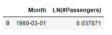
Summary and Discussion
In this blog post, we have shown how to detect anomalous points in time-series with trend and seasonality using seasonal decomposition. In general, after seasonal decomposition is applied to a given time-series, statistical tests like variance test and IQR test can then be applied to the extracted random component for anomaly/outlier detection, which can help to capture many typical anomalous points in time-series.
Seasonal decomposition model allow two types of decomposition: multiplicative and additive. Users can often see the decomposition type from the run-sequence plot of the time-series data, while the seasonal decomposition function in hana_ml can also help to determine decomposition type automatically. However, if one wants to use a specified decomposition type, appropriate data transformations are often required, otherwise the decomposition trend and seasonal components may explain the given time-series poorly.
Seasonal decomposition model allow two types of decomposition: multiplicative and additive. Users can often see the decomposition type from the run-sequence plot of the time-series data, while the seasonal decomposition function in hana_ml can also help to determine decomposition type automatically. However, if one wants to use a specified decomposition type, appropriate data transformations are often required, otherwise the decomposition trend and seasonal components may explain the given time-series poorly.
Seasonal decomposition also has some draw backs when modeling time-series, mainly illustrated as follows:
- it cannot effectively handle time-series with multiple seasonalities(e.g. weekly seasonality plus yearly seasonality)
- it becomes less efficient for modeling time-series with complicated trend
- it fails to capture cyclical but not strictly periodic fluctuations(like holidays/annual events) in time-series
- SAP Managed Tags:
- Machine Learning,
- Python,
- SAP HANA
Labels:
You must be a registered user to add a comment. If you've already registered, sign in. Otherwise, register and sign in.
Labels in this area
-
ABAP CDS Views - CDC (Change Data Capture)
2 -
AI
1 -
Analyze Workload Data
1 -
BTP
1 -
Business and IT Integration
2 -
Business application stu
1 -
Business Technology Platform
1 -
Business Trends
1,658 -
Business Trends
95 -
CAP
1 -
cf
1 -
Cloud Foundry
1 -
Confluent
1 -
Customer COE Basics and Fundamentals
1 -
Customer COE Latest and Greatest
3 -
Customer Data Browser app
1 -
Data Analysis Tool
1 -
data migration
1 -
data transfer
1 -
Datasphere
2 -
Event Information
1,400 -
Event Information
67 -
Expert
1 -
Expert Insights
177 -
Expert Insights
310 -
General
1 -
Google cloud
1 -
Google Next'24
1 -
GraphQL
1 -
Kafka
1 -
Life at SAP
780 -
Life at SAP
13 -
Migrate your Data App
1 -
MTA
1 -
Network Performance Analysis
1 -
NodeJS
1 -
PDF
1 -
POC
1 -
Product Updates
4,576 -
Product Updates
353 -
Replication Flow
1 -
REST API
1 -
RisewithSAP
1 -
SAP BTP
1 -
SAP BTP Cloud Foundry
1 -
SAP Cloud ALM
1 -
SAP Cloud Application Programming Model
1 -
SAP Datasphere
2 -
SAP S4HANA Cloud
1 -
SAP S4HANA Migration Cockpit
1 -
Technology Updates
6,873 -
Technology Updates
441 -
Workload Fluctuations
1
Related Content
- Global Explanation Capabilities in SAP HANA Machine Learning in Technology Blogs by SAP
- Fairness in Machine Learning - A New Feature in SAP HANA Cloud PAL in Technology Blogs by SAP
- Google Cloud and SAP Collaborate to Transform the Automotive Industry in Technology Blogs by SAP
- Automatic Outlier Detection for Time Series in SAP HANA in Technology Blogs by SAP
- Model Compression without Compromising Predictive Accuracy in SAP HANA PAL in Technology Blogs by SAP
Top kudoed authors
| User | Count |
|---|---|
| 20 | |
| 14 | |
| 12 | |
| 11 | |
| 10 | |
| 9 | |
| 8 | |
| 8 | |
| 7 | |
| 7 |