
- SAP Community
- Products and Technology
- Technology
- Technology Blogs by Members
- XSA Blog Series - Virtual modeling
Technology Blogs by Members
Explore a vibrant mix of technical expertise, industry insights, and tech buzz in member blogs covering SAP products, technology, and events. Get in the mix!
Turn on suggestions
Auto-suggest helps you quickly narrow down your search results by suggesting possible matches as you type.
Showing results for
MKlare
Explorer
Options
- Subscribe to RSS Feed
- Mark as New
- Mark as Read
- Bookmark
- Subscribe
- Printer Friendly Page
- Report Inappropriate Content
11-28-2023
12:14 PM
Introduction
In the fourth part of our XSA blog series we go into the details of virtual modeling and reporting. How is persistent data modeled further? Which virtual modeling options are there? Which new features do XSA Calculation Views have? How can objects be selected in other HDI containers? We will answer all these interesting questions in the following blog.
Virtual modeling basics
First, we considered the basics In the first blog with the second blog specifying the persistent structures. The third blog handled data loading so as to provide our system with content. Virtual modeling brings us into contact with old favorites from the XSC world but this time with new features.
One of the strengths of in-memory databases is virtual modeling. In contrast to classic databases, not every logic needs to be persistent to obtain good query times. Many of the common and even complex calculations can now be done on the-fly”.
For non-persistence modeling, the XSA world provides the following 4 object types as summarized in the following figure.

Fig. 1 – Virtual modeling artefacts
The following section serves as an example for the new objects. We want to join our two BillHeader and BilllItem tables and display a selection of the fields.
CDS views form part of CAP which we briefly outlined in the second blog. Involved are views based on the Core Data Services, with their own syntax and integrated in the CAP model. They can, for example, be directly saved in the schema.cds file which we created in our example project. We can directly access the corresponding associations from having saved them in our CDS model and do not need to write a Join-statement.

Fig. 2 – Example .cds view
The „cds build“ command generates the appropriate artefact which, in this case, is a .hdbview file.

Fig. 3 – Generated .hdbview
These .hdbview artefacts can also be directly written themselves. This artefact makes it possible to write „classic“ SQL and define a normal view

Fig. 4 – Example .hdbview
A table function enables the use of SQLScript and thus the use of other elements, such as IF-ELSE constructs. A drawback of the Table Functions is that the output is fixed and always needs to be specified in the correct sequence with technical name and type. The following Table Function uses the associations and only returns data on a Monday.
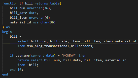
Fig. 5 – Example .hdbfunction
All 3 object types stated so far are strongly based on SQL and require appropriate prior knowledge. Moreover, optimization of these virtual objects largely depends on the developer’s know-how given that joins or calculations are carried out which may be of no importance for the actual query.
For many years now, SAP has been developing an object that is perfect for reporting purposes, namely Calculation Views. Strictly speaking, we need to talk about HDI Calculation Views at this point as they have a wider functional scope than the classic Calculation Views in the XSC environment.

Fig. 6 – Example .hdbcalculationview
We intend to look more precisely at this central and vital object type in the following section.
Calculation Views
Calculation Views are found widely in XSC systems and used, for instance, in the mixed modeling approach of a BW on HANA or BW/4HANA system. In a nutshell, Calculation Views provide nodes for graphically modeling standard functionality (projections, joins etc.). A particular feature of Calculation Views is that only the logic required by the query is carried out. This means, for instance, that whole joins or calculations can be left out if the relevant fields are not in the selection.
To consider all the features and options of Calculation Views at this stage would exceed the scope of this blog. That is why we are limiting ourselves here to a selection of new XSA features.
The following node types are currently selectable for HDI Calculation Views:
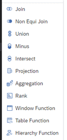
Fig, 7 – XSA node types
Those with XSC experience notice straight away that XSA has a number of new features. There is, for instance, no further limitation on Equi-Joins. As a result, Join conditions are definable with other operations as equal:

Fig. 8 – Non-Equi Joins
A highly interesting feature for performance optimization is hidden in the properties of an Inner Join:

Fig. 9 – Optimize Join Columns
Columns selected in a Join statement are always included for selection in a query even if they are not explicitly requested. Activation of the top option results in these columns also not being selected if the join is not needed. This allows for an even more pronounced aggregation of the data.
A longed for feature is the Windows functions scope. Analytical functions are involved here which are executable to a high performance on the HANA database. At one time this powerful tool was only implementable as Table Functions to be then incorporated in Calculation Views as projection.
Thanks to the „Window Function“ node, they are now directly executable in a Calculation View. All functions are available in the update and the relevant parameters can be graphically updated:

Fig. 10 – Window Function example
Debugging represents a major challenge in working with SQL. In contrast to imperative languages, an SQL statement has no loops or step-wise statements. A statement is either fully executed or not at all. That is why looking for errors is difficult particularly with complex and nested views. For this the Calculation View provides a practical feature: the Debug View

Fig. 11 – Start Debug
A click on this option opens up a new tab in the Debug Query properties

Fig. 12 – Generated Debug SQL
This tab firstly comprises a generated SQL statement which with the appropriate button is executable. At first glance it does not seem to be a particular feature – the Data Explorer can also be used to execute a SQL statement onto a view. It is only when clicking a sub-node in the Calculation View that the particular feature is noticed. The Debug Query tab is now also available in this sub-node.

Fig. 13 – Debug nodes
Views for the individual nodes, which always follow the name convention “[Name of the Calculation View]/dp/[Name of the node]” are generated in the background. It thus becomes convenient to select and analyze all sub-findings of the nodes. This, in classic XSC, was only possible via detours and Data Previews – but not directly in the IDE.
All virtual objects initially only have access to those tables and views which exist in their own HDI container. But how can objects be selected which exist in other HDI containers? The isolated architecture of HDI containers makes this possible only with new artefacts and a manual steps.
Cross-Access HDI Container
In this section we want to show how objects in another HDI container can be accessed. Recap: a HDI container represents an isolated area on the database which essentially only knows about itself. No other HDI containers and their objects are visible. In our example we have the source HDI container (HDI_SOURCE) which wants to read a table from the target HDI container (HDI_TARGET). The following illustration shows the setup for cross-access with HDI containers
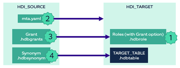
Fig. 14 – Cross-Access procedure
The following steps are needed:
- Creating roles (.hdbrole) in HDI_TARGET
- Connecting the HDI containers from adjustment to mta.yaml in HDI_SOURCE
- Creating Grant (.hdbgrants) for reading out the roles
- Creating Synonym for target object
This rather complex approach is the result of HDI container isolation. The HDI container (HDI_TARGET) firstly needs to define roles which permit access to its objects. The source container (HDI_SOURCE) uses a Grant artefact to incorporate these roles. Unfortunately, it is not possible to directly access the objects. Every object needs a “synonym” which can then, for instance, be used in a Calculation View.
A practical tip: many of the artefacts have their own graphical updating dialog. However, all files can be directly edited with a right click via the Text Editor.

Fig. 15 – Updating in Text Edito
We have created an appropriate HDI container with a table

Fig. 16 – Target table in HDI_TARGET
For access, we generate the required roles in the roles folder:

Fig. 17 – Example .hdbrole without Grant

Fig. 18 – Example .hdbrole with Grant
There is now the question of why two roles are needed. The second role in its technical name has a hashtag (#) and via “Grant Option” assigns rights which, as a result, can be passed on. This two-role interplay is a technical necessity since an HDI consists of several users. The role without Grant is assigned to the _RT User (Application User), the _OO (Object Owner) User obtains the role with Grant. This role can, of course, be limited even further. In our case, reading and writing rights are assigned to all objects in the HDI container. These roles firstly need to be deployed before our HDI container can access them.
Now 3 steps need to be carried out in our XSA blog project. First of all, we update the target HDI container in the central control file (mta.yaml). Whilst this theoretically can be manually inputted, BAS provides a convenient option here in the GUI:
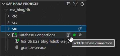
Fig. 19 – Connection HDI Container (1/2)
The required HDI container can simply be selected in the now-opened window:

Fig. 20 – Connection HDI Container (2/2)
In this way, the mta.yaml file is automatically adjusted. In addition, the .env file in the db folder is extended by the appropriate service.
The second step is creating the Grants file in the “cfg” folder:

Fig. 21 – Example .hdbrole
In this file, the appropriate roles are assigned to the Application User and Object Owner.
Both the HDI containers are now connected and the required rights and roles created. The synonyms need to be updated in the third and final step. Every object that is to be read from the target HDI container must be named in the synonym file.

Fig. 22 – Example .hdbsynonym
The object can now be directly used in our Calculation View.

Fig. 23 – Synonym in Calculation View
As mentioned in the second blog, the isolated HDI containers provide for greater focusing on the design. The decision on which objects are to be in an HDI container and which dependencies exist has a prime role to play in XSA. In this connection, the following facts are important in a design:
- An HDI container can only be deployed as a whole (with all its objects)
- Target objects from an HDI container have no connection to their use as synonyms. An error develops solely in the reading HDI container
- Connections of HDI containers result in dependencies with the Deployment since the object referencing the Synonym must always exist
Summary
XSA reveals its full potential in virtual modeling. Depending on application and know-how, the different artefacts enable the right tools to be selected. In particular, the performance and debugging scope of the Calculation View catch the eye.
The only downside is the connection of various HDI containers. The isolated HDI containers explain why it is necessary to have several manual adjustments and diverse artefacts. Especially with large Data Warehouse applications, updating a synonym for each new object is somewhat obstructive.
We deal with NodeJS in the fifth and final part of our blog series. Integration of NodeJS in XSA allows complex services to be developed which with pure database means and SQL would not be possible.
- SAP Managed Tags:
- SAP HANA Cloud,
- Data and Analytics,
- SAP HANA
You must be a registered user to add a comment. If you've already registered, sign in. Otherwise, register and sign in.
Labels in this area
-
"automatische backups"
1 -
"regelmäßige sicherung"
1 -
"TypeScript" "Development" "FeedBack"
1 -
505 Technology Updates 53
1 -
ABAP
14 -
ABAP API
1 -
ABAP CDS Views
2 -
ABAP CDS Views - BW Extraction
1 -
ABAP CDS Views - CDC (Change Data Capture)
1 -
ABAP class
2 -
ABAP Cloud
3 -
ABAP Development
5 -
ABAP in Eclipse
1 -
ABAP Platform Trial
1 -
ABAP Programming
2 -
abap technical
1 -
abapGit
1 -
absl
2 -
access data from SAP Datasphere directly from Snowflake
1 -
Access data from SAP datasphere to Qliksense
1 -
Accrual
1 -
action
1 -
adapter modules
1 -
Addon
1 -
Adobe Document Services
1 -
ADS
1 -
ADS Config
1 -
ADS with ABAP
1 -
ADS with Java
1 -
ADT
2 -
Advance Shipping and Receiving
1 -
Advanced Event Mesh
3 -
Advanced formula
1 -
AEM
1 -
AI
7 -
AI Launchpad
1 -
AI Projects
1 -
AIML
9 -
Alert in Sap analytical cloud
1 -
Amazon S3
1 -
Analytical Dataset
1 -
Analytical Model
1 -
Analytics
1 -
Analyze Workload Data
1 -
annotations
1 -
API
1 -
API and Integration
3 -
API Call
2 -
API security
1 -
Application Architecture
1 -
Application Development
5 -
Application Development for SAP HANA Cloud
3 -
Applications and Business Processes (AP)
1 -
Artificial Intelligence
1 -
Artificial Intelligence (AI)
5 -
Artificial Intelligence (AI) 1 Business Trends 363 Business Trends 8 Digital Transformation with Cloud ERP (DT) 1 Event Information 462 Event Information 15 Expert Insights 114 Expert Insights 76 Life at SAP 418 Life at SAP 1 Product Updates 4
1 -
Artificial Intelligence (AI) blockchain Data & Analytics
1 -
Artificial Intelligence (AI) blockchain Data & Analytics Intelligent Enterprise
1 -
Artificial Intelligence (AI) blockchain Data & Analytics Intelligent Enterprise Oil Gas IoT Exploration Production
1 -
Artificial Intelligence (AI) blockchain Data & Analytics Intelligent Enterprise sustainability responsibility esg social compliance cybersecurity risk
1 -
ASE
1 -
ASR
2 -
ASUG
1 -
Attachments
1 -
Authorisations
1 -
Automating Processes
1 -
Automation
2 -
aws
2 -
Azure
1 -
Azure AI Studio
1 -
Azure API Center
1 -
Azure API Management
1 -
B2B Integration
1 -
Backorder Processing
1 -
Backup
1 -
Backup and Recovery
1 -
Backup schedule
1 -
BADI_MATERIAL_CHECK error message
1 -
Bank
1 -
Bank Communication Management
1 -
BAS
1 -
basis
2 -
Basis Monitoring & Tcodes with Key notes
2 -
Batch Management
1 -
BDC
1 -
Best Practice
1 -
bitcoin
1 -
Blockchain
3 -
bodl
1 -
BOP in aATP
1 -
BOP Segments
1 -
BOP Strategies
1 -
BOP Variant
1 -
BPC
1 -
BPC LIVE
1 -
BTP
13 -
BTP AI Launchpad
1 -
BTP Destination
2 -
Business AI
1 -
Business and IT Integration
1 -
Business application stu
1 -
Business Application Studio
1 -
Business Architecture
1 -
Business Communication Services
1 -
Business Continuity
1 -
Business Data Fabric
3 -
Business Fabric
1 -
Business Partner
12 -
Business Partner Master Data
10 -
Business Technology Platform
2 -
Business Trends
4 -
BW4HANA
1 -
CA
1 -
calculation view
1 -
CAP
4 -
Capgemini
1 -
CAPM
1 -
Catalyst for Efficiency: Revolutionizing SAP Integration Suite with Artificial Intelligence (AI) and
1 -
CCMS
2 -
CDQ
12 -
CDS
2 -
Cental Finance
1 -
Certificates
1 -
CFL
1 -
Change Management
1 -
chatbot
1 -
chatgpt
3 -
CL_SALV_TABLE
2 -
Class Runner
1 -
Classrunner
1 -
Cloud ALM Monitoring
1 -
Cloud ALM Operations
1 -
cloud connector
1 -
Cloud Extensibility
1 -
Cloud Foundry
4 -
Cloud Integration
6 -
Cloud Platform Integration
2 -
cloudalm
1 -
communication
1 -
Compensation Information Management
1 -
Compensation Management
1 -
Compliance
1 -
Compound Employee API
1 -
Configuration
1 -
Connectors
1 -
Consolidation Extension for SAP Analytics Cloud
2 -
Control Indicators.
1 -
Controller-Service-Repository pattern
1 -
Conversion
1 -
Cosine similarity
1 -
cryptocurrency
1 -
CSI
1 -
ctms
1 -
Custom chatbot
3 -
Custom Destination Service
1 -
custom fields
1 -
Customer Experience
1 -
Customer Journey
1 -
Customizing
1 -
cyber security
3 -
cybersecurity
1 -
Data
1 -
Data & Analytics
1 -
Data Aging
1 -
Data Analytics
2 -
Data and Analytics (DA)
1 -
Data Archiving
1 -
Data Back-up
1 -
Data Flow
1 -
Data Governance
5 -
Data Integration
2 -
Data Quality
12 -
Data Quality Management
12 -
Data Synchronization
1 -
data transfer
1 -
Data Unleashed
1 -
Data Value
8 -
database tables
1 -
Dataframe
1 -
Datasphere
3 -
datenbanksicherung
1 -
dba cockpit
1 -
dbacockpit
1 -
Debugging
2 -
Defender
1 -
Delimiting Pay Components
1 -
Delta Integrations
1 -
Destination
3 -
Destination Service
1 -
Developer extensibility
1 -
Developing with SAP Integration Suite
1 -
Devops
1 -
digital transformation
1 -
Documentation
1 -
Dot Product
1 -
DQM
1 -
dump database
1 -
dump transaction
1 -
e-Invoice
1 -
E4H Conversion
1 -
Eclipse ADT ABAP Development Tools
2 -
edoc
1 -
edocument
1 -
ELA
1 -
Embedded Consolidation
1 -
Embedding
1 -
Embeddings
1 -
Employee Central
1 -
Employee Central Payroll
1 -
Employee Central Time Off
1 -
Employee Information
1 -
Employee Rehires
1 -
Enable Now
1 -
Enable now manager
1 -
endpoint
1 -
Enhancement Request
1 -
Enterprise Architecture
1 -
ESLint
1 -
ETL Business Analytics with SAP Signavio
1 -
Euclidean distance
1 -
Event Dates
1 -
Event Driven Architecture
1 -
Event Mesh
2 -
Event Reason
1 -
EventBasedIntegration
1 -
EWM
1 -
EWM Outbound configuration
1 -
EWM-TM-Integration
1 -
Existing Event Changes
1 -
Expand
1 -
Expert
2 -
Expert Insights
2 -
Exploits
1 -
Fiori
14 -
Fiori Elements
2 -
Fiori SAPUI5
12 -
first-guidance
1 -
Flask
1 -
FTC
1 -
Full Stack
8 -
Funds Management
1 -
gCTS
1 -
GenAI hub
1 -
General
1 -
Generative AI
1 -
Getting Started
1 -
GitHub
9 -
Grants Management
1 -
groovy
1 -
GTP
1 -
HANA
6 -
HANA Cloud
2 -
Hana Cloud Database Integration
2 -
HANA DB
2 -
Hana Vector Engine
1 -
HANA XS Advanced
1 -
Historical Events
1 -
home labs
1 -
HowTo
1 -
HR Data Management
1 -
html5
8 -
HTML5 Application
1 -
Identity cards validation
1 -
idm
1 -
Implementation
1 -
Infuse AI
1 -
input parameter
1 -
instant payments
1 -
Integration
3 -
Integration Advisor
1 -
Integration Architecture
1 -
Integration Center
1 -
Integration Suite
1 -
intelligent enterprise
1 -
iot
1 -
Java
1 -
job
1 -
Job Information Changes
1 -
Job-Related Events
1 -
Job_Event_Information
1 -
joule
4 -
Journal Entries
1 -
Just Ask
1 -
Kerberos for ABAP
8 -
Kerberos for JAVA
8 -
KNN
1 -
Launch Wizard
1 -
Learning Content
2 -
Life at SAP
5 -
lightning
1 -
Linear Regression SAP HANA Cloud
1 -
Loading Indicator
1 -
local tax regulations
1 -
LP
1 -
Machine Learning
3 -
Marketing
1 -
Master Data
3 -
Master Data Management
14 -
Maxdb
2 -
MDG
1 -
MDGM
1 -
MDM
1 -
Message box.
1 -
Messages on RF Device
1 -
Microservices Architecture
1 -
Microsoft Universal Print
1 -
Middleware Solutions
1 -
Migration
5 -
ML Model Development
1 -
Modeling in SAP HANA Cloud
8 -
Monitoring
3 -
MTA
1 -
Multi-Record Scenarios
1 -
Multiple Event Triggers
1 -
Myself Transformation
1 -
Neo
1 -
New Event Creation
1 -
New Feature
1 -
Newcomer
1 -
NodeJS
3 -
ODATA
2 -
OData APIs
1 -
odatav2
1 -
ODATAV4
1 -
ODBC
1 -
ODBC Connection
1 -
Onpremise
1 -
open source
2 -
OpenAI API
1 -
Oracle
1 -
PaPM
1 -
PaPM Dynamic Data Copy through Writer function
1 -
PaPM Remote Call
1 -
Partner Built Foundation Model
1 -
PAS-C01
1 -
Pay Component Management
1 -
PGP
1 -
Pickle
1 -
PLANNING ARCHITECTURE
1 -
Popup in Sap analytical cloud
1 -
PostgrSQL
1 -
POSTMAN
1 -
Prettier
1 -
Process Automation
2 -
Product Updates
6 -
PSM
1 -
Public Cloud
1 -
Python
4 -
python library - Document information extraction service
1 -
Qlik
1 -
Qualtrics
1 -
RAP
3 -
RAP BO
2 -
Record Deletion
1 -
Recovery
1 -
recurring payments
1 -
redeply
1 -
Release
1 -
Remote Consumption Model
1 -
Replication Flows
1 -
research
1 -
Resilience
1 -
REST
1 -
REST API
1 -
Retagging Required
1 -
Risk
1 -
Rolling Kernel Switch
1 -
route
1 -
rules
1 -
S4 HANA
1 -
S4 HANA Cloud
1 -
S4 HANA On-Premise
1 -
S4HANA
3 -
S4HANA_OP_2023
2 -
SAC
10 -
SAC PLANNING
9 -
SAP
4 -
SAP ABAP
1 -
SAP Advanced Event Mesh
1 -
SAP AI Core
9 -
SAP AI Launchpad
8 -
SAP Analytic Cloud Compass
1 -
Sap Analytical Cloud
1 -
SAP Analytics Cloud
4 -
SAP Analytics Cloud for Consolidation
3 -
SAP Analytics Cloud Story
1 -
SAP analytics clouds
1 -
SAP API Management
1 -
SAP BAS
1 -
SAP Basis
6 -
SAP BODS
1 -
SAP BODS certification.
1 -
SAP BTP
21 -
SAP BTP Build Work Zone
2 -
SAP BTP Cloud Foundry
6 -
SAP BTP Costing
1 -
SAP BTP CTMS
1 -
SAP BTP Generative AI
1 -
SAP BTP Innovation
1 -
SAP BTP Migration Tool
1 -
SAP BTP SDK IOS
1 -
SAP BTPEA
1 -
SAP Build
11 -
SAP Build App
1 -
SAP Build apps
1 -
SAP Build CodeJam
1 -
SAP Build Process Automation
3 -
SAP Build work zone
10 -
SAP Business Objects Platform
1 -
SAP Business Technology
2 -
SAP Business Technology Platform (XP)
1 -
sap bw
1 -
SAP CAP
2 -
SAP CDC
1 -
SAP CDP
1 -
SAP CDS VIEW
1 -
SAP Certification
1 -
SAP Cloud ALM
4 -
SAP Cloud Application Programming Model
1 -
SAP Cloud Integration for Data Services
1 -
SAP cloud platform
8 -
SAP Companion
1 -
SAP CPI
3 -
SAP CPI (Cloud Platform Integration)
2 -
SAP CPI Discover tab
1 -
sap credential store
1 -
SAP Customer Data Cloud
1 -
SAP Customer Data Platform
1 -
SAP Data Intelligence
1 -
SAP Data Migration in Retail Industry
1 -
SAP Data Services
1 -
SAP DATABASE
1 -
SAP Dataspher to Non SAP BI tools
1 -
SAP Datasphere
9 -
SAP DRC
1 -
SAP EWM
1 -
SAP Fiori
3 -
SAP Fiori App Embedding
1 -
Sap Fiori Extension Project Using BAS
1 -
SAP GRC
1 -
SAP HANA
1 -
SAP HANA Vector
1 -
SAP HCM (Human Capital Management)
1 -
SAP HR Solutions
1 -
SAP IDM
1 -
SAP Integration Suite
9 -
SAP Integrations
4 -
SAP iRPA
2 -
SAP LAGGING AND SLOW
1 -
SAP Learning Class
1 -
SAP Learning Hub
1 -
SAP Master Data
1 -
SAP Odata
2 -
SAP on Azure
2 -
SAP PAL
1 -
SAP PartnerEdge
1 -
sap partners
1 -
SAP Password Reset
1 -
SAP PO Migration
1 -
SAP Prepackaged Content
1 -
SAP Process Automation
2 -
SAP Process Integration
2 -
SAP Process Orchestration
1 -
SAP S4HANA
2 -
SAP S4HANA Cloud
1 -
SAP S4HANA Cloud for Finance
1 -
SAP S4HANA Cloud private edition
1 -
SAP Sandbox
1 -
SAP STMS
1 -
SAP successfactors
3 -
SAP SuccessFactors HXM Core
1 -
SAP Time
1 -
SAP TM
2 -
SAP Trading Partner Management
1 -
SAP UI5
1 -
SAP Upgrade
1 -
SAP Utilities
1 -
SAP-GUI
8 -
SAP_COM_0276
1 -
SAPBTP
1 -
SAPCPI
1 -
SAPEWM
1 -
sapfirstguidance
1 -
SAPHANAService
1 -
SAPIQ
1 -
sapmentors
1 -
saponaws
2 -
SAPS4HANA
1 -
SAPUI5
5 -
schedule
1 -
Script Operator
1 -
Secure Login Client Setup
8 -
security
9 -
Selenium Testing
1 -
Self Transformation
1 -
Self-Transformation
1 -
SEN
1 -
SEN Manager
1 -
service
1 -
SET_CELL_TYPE
1 -
SET_CELL_TYPE_COLUMN
1 -
SFTP scenario
2 -
Simplex
1 -
Single Sign On
8 -
Singlesource
1 -
SKLearn
1 -
Slow loading
1 -
soap
1 -
Software Development
1 -
SOLMAN
1 -
solman 7.2
2 -
Solution Manager
3 -
sp_dumpdb
1 -
sp_dumptrans
1 -
SQL
1 -
sql script
1 -
SSL
8 -
SSO
8 -
Substring function
1 -
SuccessFactors
1 -
SuccessFactors Platform
1 -
SuccessFactors Time Tracking
1 -
Sybase
1 -
system copy method
1 -
System owner
1 -
Table splitting
1 -
Tax Integration
1 -
Technical article
1 -
Technical articles
1 -
Technology Updates
15 -
Technology Updates
1 -
Technology_Updates
1 -
terraform
1 -
Threats
2 -
Time Collectors
1 -
Time Off
2 -
Time Sheet
1 -
Time Sheet SAP SuccessFactors Time Tracking
1 -
Tips and tricks
2 -
toggle button
1 -
Tools
1 -
Trainings & Certifications
1 -
Transformation Flow
1 -
Transport in SAP BODS
1 -
Transport Management
1 -
TypeScript
3 -
ui designer
1 -
unbind
1 -
Unified Customer Profile
1 -
UPB
1 -
Use of Parameters for Data Copy in PaPM
1 -
User Unlock
1 -
VA02
1 -
Validations
1 -
Vector Database
2 -
Vector Engine
1 -
Vectorization
1 -
Visual Studio Code
1 -
VSCode
2 -
VSCode extenions
1 -
Vulnerabilities
1 -
Web SDK
1 -
work zone
1 -
workload
1 -
xsa
1 -
XSA Refresh
1
- « Previous
- Next »
Related Content
- Quick & Easy Datasphere - When to use Data Flow, Transformation Flow, SQL View? in Technology Blogs by Members
- Exploring Integration Options in SAP Datasphere with the focus on using SAP extractors - Part II in Technology Blogs by SAP
- Best Practice: How to Structure the Shared Document Folder in Technology Blogs by SAP
- Top Picks: Innovations Highlights from SAP Business Technology Platform (Q1/2024) in Technology Blogs by SAP
- SAP Sustainability Footprint Management: Q1-24 Updates & Highlights in Technology Blogs by SAP
Top kudoed authors
| User | Count |
|---|---|
| 10 | |
| 9 | |
| 5 | |
| 4 | |
| 4 | |
| 4 | |
| 3 | |
| 3 | |
| 3 | |
| 3 |