
- SAP Community
- Products and Technology
- Enterprise Resource Planning
- ERP Blogs by SAP
- CDS View Performance Best Practice – NOT NULL pres...
Enterprise Resource Planning Blogs by SAP
Get insights and updates about cloud ERP and RISE with SAP, SAP S/4HANA and SAP S/4HANA Cloud, and more enterprise management capabilities with SAP blog posts.
Turn on suggestions
Auto-suggest helps you quickly narrow down your search results by suggesting possible matches as you type.
Showing results for
Advisor
Options
- Subscribe to RSS Feed
- Mark as New
- Mark as Read
- Bookmark
- Subscribe
- Printer Friendly Page
- Report Inappropriate Content
11-02-2023
3:14 PM
This blog post focuses on the CDS view performance anti-pattern called "NOT NULL preserving LEFT OUTER JOIN" and it's part of the CDS View Performance Best Practices series. You can find an introduction to CDS View performance recommendations, aspects you need to consider in terms of performance, and a list of all available CDS anti-patterns in the following blog post: https://blogs.sap.com/2023/06/26/cds-view-performance-best-practises/
The "NOT NULL preserving LEFT OUTER JOIN" is one of the most prominent anti-patterns, which can cause very severe performance problems. Let us see with a simple example how exactly you can identify this anti-pattern, the impact and why this leads to a performance problem.
What is meant by “preserve NOT NULL” exactly? It is a calculation which will never have NULL as a result.
This calculation (Fig. 1) returns the value X if the condition is true. In all other scenarios the result will be a blank value. So, it will never return NULL. Let’s demonstrate the result of this calculation with different input values for the expression (Fig. 2).
This pattern is also valid for other functions:
Additionally keep in mind that functions can have an implicit default result of NULL if no expressions are fulfilled. In our scenario this is overwritten by the ELSE branch. This is by itself not bad or an anti-pattern, but it causes a big performance problem when the calculation is part of a LEFT OUTER JOIN, which is the case for association in the model. Why is this a problem?
Basically, as soon as you have a field which doesn’t preserve the NULL behavior, the SAP HANA optimizer first needs to execute the calculation for every row (even for the rows which are discarded after the left outer join) and build up an intermediate result set to guarantee functional correctness and then execute the join. This is the key message of this blog post and anti-pattern to understand the NULL handling in SQL.
Let's imagine an example of two models (Fig. 3) and would like to return the result shown in Fig. 4. So, we have one model for order items, the purchase order items, and another model for order header, the purchase document (Fig. 6). This model will be used in the purchase order items model to get the status of the order and contain a calculated field. Additionally, we apply a filter on a specific material TG11 to reduce the amount of data (Fig. 5).
The purchase document is joined via an association as a one to one relation in our model (Fig. 7) which will be generated as a LEFT OUTER JOIN with the cardinality MANY TO ONE (Fig. 😎. Keep in mind that in our example we do not have any foreign key constraints set up on the SAP HANA database schema for our tables. Therefore, the database does not know any relation between our tables and has only the information contained in the join definition.
First start with a simple query with fields in the projection list, which are only from one single table (order item) of our model to compare afterwards the performance and see the impact.
The execution finished quite fast in just 5ms (Fig. 9).
The PlanViz (Fig. 10) shows only one column search operator with filter push down to one relation which results in small intermediate result set and therefore fast data processing for subsequent plan operators.
Let’s now add an additional field “enjoyReleaseNotCompleted” to the projection list and leave the remaining part of statement as it is. The query execution time went up to more than 2 seconds (Fig. 11).
In the PlanViz we can see now a high intermediate result set and stacked column search operators (Fig. 12). In the operator details of the first column search operator, we can see the calculation (CASE function) on an unfiltered table, which means that the calculation was executed for all rows of the table. This is the root cause of the increased runtime and bad performance. Afterwards this intermediate result is joined with the other table, where filter push was working properly.
So, what is wrong with this field and why does it have such a high impact on our query execution? Why can’t the filter be applied already before or the calculation executed after the filter have been applied? The problem is related to the left outer join (association) of the purchase document model, which contains the calculated field ”enjoyReleaseNotCompleted”. (Fig. 13)
The SAP HANA optimizer first needs to execute the calculation on the purchase document view (Fig. 14) as it’s joined via a LEFT OUTER JOIN to the purchase order item. Since this needs to be executed for all purchase orders it might require high number of resources and could lead to big intermediate results, high memory consumption and high execution duration of the sub plan operation depending on data amount in the relation. The filter on material can’t be applied as we don’t have a material on this model. Please, watch out that the header don't have a record for the order NNN.
Then execute the (left outer) join on top of the intermediate result with the calculated value (see Fig. 15). This results into a NULL value for the order NNN as we don't have a matched record in the order header.
Let’s have a look at how the result would look like if the optimizer would exchange the sequence of the operation by first doing the left outer join (Fig. 16) and then afterwards ("at the end”) execute the calculation (Fig. 17) on top of the result of this join.
Now you see what happens, the result of the calculated field "enjoyReleaseNotCompleted" is different and leads to a blank value for the order NNN due to the ELSE branch in the calculation. That’s an issue, because the optimizer can only reorder operators if it still returns exactly the same result. This exchange of operators is therefore not allowed by the optimizer.
Since the left outer join will create NULL values for entries of purchase orders, where no matching order header records exist, the case expression on top will calculate a value which is NOT NULL, a blank value. However, this is wrong and not allowed by SAP HANA Optimizer, since the calculation is defined as part of the right side on a LEFT OUTER JOIN and so values not equal to NULL must only exist for items with a matching header record.
In the comparison (Fig. 18) of both results you can see the outputs of the calculation are different, highlighted in yellow.
In case we have a pretty selective filter in the purchase order items, e.g. only in-complete purchase order items of a single vendor, from performance perspective it would be the best option to first join and then do the calculation, but since the results would be potentially wrong, the SAP HANA optimizer is not allowed to exchange the order of the join and the calculation.
To avoid the materialization of a large intermediate result set on SAP HANA and have better performance you have different options. Let's start with the first option by changing the model and then afterwards I will explain a second option.
One option to improve this performance problem is to remove the not null preserving function. This can be done for instance by removing the ELSE branch from the calculation. Then it returns NULL if the condition is not fulfilled.
Execute the query by using a new column in the projection results in just 10ms execution duration.
Once you make this code change a warning message (Fig. 21) is displayed in ADT (ABAP Development Tool) saying that a missing ELSE branch lead to NULL values.
This is an important message as the code change results in a slight semantical difference in the result. The NULL output needs to be covered in the upper view stack or application.
Following you will see the PlanViz with the optimized calculation. In this specific query the filter, join, order by and limit can be applied before the calculation is executed and so the overall execution is much more efficient.
Another option to mitigate the problem would be to rewrite the expression of the ELSE branch to a NULL preserving expression by adding a second expression with the inverted condition and omitting the ELSE argument (Fig. 23). This condition excludes the NULL value expression as the ELSE argument is optional. The NULL "value" is not explicit handled anymore, but will be implicit evaluated by the Optimizer.
With SAP HANA 2.0 SPS7 this anti-pattern is considered in HEX, which avoids high intermediate result sets and is covered in the execution plan generation. This means that no changes to the data model or statement implementation by the application are required. Instead, it will be automatically considered as soon as the HEX engine is used for the query.

Let me explain this PlanViz in more detail showing the intermediate results of the execution plan for our example which explains what the SAP HANA is actually doing and how the semi join reduction works.
The first step (Step 1) is the filter on order items (Fig. 25) for material TG11 which reduces the data amount significantly. This result (Step 2) will be used in the subsequent steps.
Now, a semi join is executed by creating a unique order list for each join partner, the orders items and order headers. So, it creates an intermediate result for all orders in order items which have at least one match in the header, the intersection (Fig. 26).
On this result the calculation will then be executed (see Step 4 - Fig. 27). Which means that in our example the order NNN and MNO won’t be part of our so-called purchase document as no matching record exists either in the items or in the header table. The SQL “SELECT * FROM A WHERE A.key IN (SELECT B.key from B)” would be the equivalent SQL expression.
In the final step 5 (Fig. 28) after the semi join the result from step 2 (applied filter) will be joined (via LEFT OUTER) with the result of step 4 (calculation).
In the result (Fig. 28) now you can see that only for the order items ABC and XYZ the calculation gives a valid value. The calculation for order item NNN was not executed (MNO was removed by the filter on material) and that’s why NULL has to be shown due to the LEFT OUTER JOIN.
It’s a great new feature and performance improvement in HEX made available in the latest release of SAP HANA 2 which can be leveraged in different scenarios automatically without any changes to the model or application. However, it is still beneficial to remove the not null preserving pattern from your application model since this kind of transformation explained here requires two joins instead of one. E.g., in situations where no selective filter is applied the better choice would be to do the calculation on all items to avoid the additional semi join. Whether the semi join is used or not is decided by the optimizer based on estimated query costs and this of course increases the complexity of the query compilation, which in turn makes it harder to find a good execution plan and therefore increases compile times which may increases the risk that a sub-optimal execution plan is chosen.
The "NOT NULL preserving LEFT OUTER JOIN" is one of the most prominent anti-patterns, which can cause very severe performance problems. Let us see with a simple example how exactly you can identify this anti-pattern, the impact and why this leads to a performance problem.
What is meant by “preserve NOT NULL” exactly? It is a calculation which will never have NULL as a result.

Figure 1: not null preserving calculation
This calculation (Fig. 1) returns the value X if the condition is true. In all other scenarios the result will be a blank value. So, it will never return NULL. Let’s demonstrate the result of this calculation with different input values for the expression (Fig. 2).

Figure 2: different scenarios for calculation
This pattern is also valid for other functions:
- COALESCE – default parameter
- CASE … ELSE <another CASE>
- <constant> – a fixed value
Additionally keep in mind that functions can have an implicit default result of NULL if no expressions are fulfilled. In our scenario this is overwritten by the ELSE branch. This is by itself not bad or an anti-pattern, but it causes a big performance problem when the calculation is part of a LEFT OUTER JOIN, which is the case for association in the model. Why is this a problem?
Basically, as soon as you have a field which doesn’t preserve the NULL behavior, the SAP HANA optimizer first needs to execute the calculation for every row (even for the rows which are discarded after the left outer join) and build up an intermediate result set to guarantee functional correctness and then execute the join. This is the key message of this blog post and anti-pattern to understand the NULL handling in SQL.
Example
Let's imagine an example of two models (Fig. 3) and would like to return the result shown in Fig. 4. So, we have one model for order items, the purchase order items, and another model for order header, the purchase document (Fig. 6). This model will be used in the purchase order items model to get the status of the order and contain a calculated field. Additionally, we apply a filter on a specific material TG11 to reduce the amount of data (Fig. 5).

Figure 3: example overview of models

Figure 4: expected result for given example

Figure 5: items filtered on one material TG11

Figure 6: purchase document with calculation
The purchase document is joined via an association as a one to one relation in our model (Fig. 7) which will be generated as a LEFT OUTER JOIN with the cardinality MANY TO ONE (Fig. 😎. Keep in mind that in our example we do not have any foreign key constraints set up on the SAP HANA database schema for our tables. Therefore, the database does not know any relation between our tables and has only the information contained in the join definition.

Figure 7: Model of purchase order item with association to purchase document

Figure 8: snippet of SQL DDL artifact for association
First start with a simple query with fields in the projection list, which are only from one single table (order item) of our model to compare afterwards the performance and see the impact.
SELECT  purchaseorder, purchaseorderitem, material

FROM    ZRW_PURCHORDRITEM

WHERE   material = ?

ORDER BY purchaseorder, purchaseorderitem

LIMIT 200;
The execution finished quite fast in just 5ms (Fig. 9).

Figure 9: execution time (fast) without calculated field
The PlanViz (Fig. 10) shows only one column search operator with filter push down to one relation which results in small intermediate result set and therefore fast data processing for subsequent plan operators.

Figure 10: PlanViz without calculated field
Let’s now add an additional field “enjoyReleaseNotCompleted” to the projection list and leave the remaining part of statement as it is. The query execution time went up to more than 2 seconds (Fig. 11).

Figure 11: execution time (slow) with calculated field
In the PlanViz we can see now a high intermediate result set and stacked column search operators (Fig. 12). In the operator details of the first column search operator, we can see the calculation (CASE function) on an unfiltered table, which means that the calculation was executed for all rows of the table. This is the root cause of the increased runtime and bad performance. Afterwards this intermediate result is joined with the other table, where filter push was working properly.

Figure 12: PlanViz with high intermediate result set
So, what is wrong with this field and why does it have such a high impact on our query execution? Why can’t the filter be applied already before or the calculation executed after the filter have been applied? The problem is related to the left outer join (association) of the purchase document model, which contains the calculated field ”enjoyReleaseNotCompleted”. (Fig. 13)
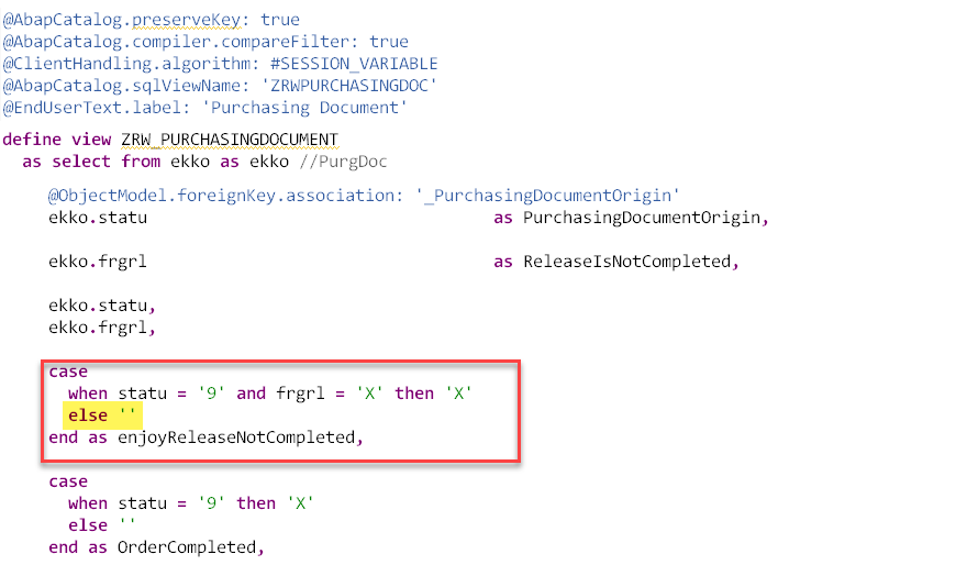
Figure 13: model with NOT NULL preserving calculation
The SAP HANA optimizer first needs to execute the calculation on the purchase document view (Fig. 14) as it’s joined via a LEFT OUTER JOIN to the purchase order item. Since this needs to be executed for all purchase orders it might require high number of resources and could lead to big intermediate results, high memory consumption and high execution duration of the sub plan operation depending on data amount in the relation. The filter on material can’t be applied as we don’t have a material on this model. Please, watch out that the header don't have a record for the order NNN.

Figure 14: Step 1 - calculate first
Then execute the (left outer) join on top of the intermediate result with the calculated value (see Fig. 15). This results into a NULL value for the order NNN as we don't have a matched record in the order header.

Figure 15: Step 2 - join (left outer), after calculation
Let’s have a look at how the result would look like if the optimizer would exchange the sequence of the operation by first doing the left outer join (Fig. 16) and then afterwards ("at the end”) execute the calculation (Fig. 17) on top of the result of this join.

Figure 16: exchange operators - Step 1 - join (left outer) first

Figure 17: exchange operators - Step 2 - afterwards execute calculation
Now you see what happens, the result of the calculated field "enjoyReleaseNotCompleted" is different and leads to a blank value for the order NNN due to the ELSE branch in the calculation. That’s an issue, because the optimizer can only reorder operators if it still returns exactly the same result. This exchange of operators is therefore not allowed by the optimizer.
Since the left outer join will create NULL values for entries of purchase orders, where no matching order header records exist, the case expression on top will calculate a value which is NOT NULL, a blank value. However, this is wrong and not allowed by SAP HANA Optimizer, since the calculation is defined as part of the right side on a LEFT OUTER JOIN and so values not equal to NULL must only exist for items with a matching header record.
In the comparison (Fig. 18) of both results you can see the outputs of the calculation are different, highlighted in yellow.
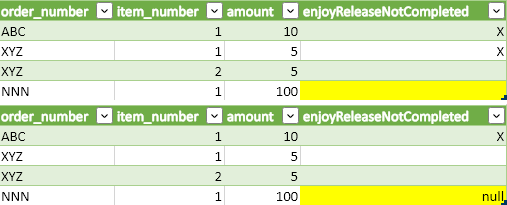
Figure 18: comparison of exchanged operators
In case we have a pretty selective filter in the purchase order items, e.g. only in-complete purchase order items of a single vendor, from performance perspective it would be the best option to first join and then do the calculation, but since the results would be potentially wrong, the SAP HANA optimizer is not allowed to exchange the order of the join and the calculation.
Possible Solution
To avoid the materialization of a large intermediate result set on SAP HANA and have better performance you have different options. Let's start with the first option by changing the model and then afterwards I will explain a second option.
One option to improve this performance problem is to remove the not null preserving function. This can be done for instance by removing the ELSE branch from the calculation. Then it returns NULL if the condition is not fulfilled.

Figure 19: Calculation - preserve NULLs
Execute the query by using a new column in the projection results in just 10ms execution duration.

Figure 20: execution duration without ELSE branch
Once you make this code change a warning message (Fig. 21) is displayed in ADT (ABAP Development Tool) saying that a missing ELSE branch lead to NULL values.

Figure 21: ADT warning message on CASE function without ELSE branch
This is an important message as the code change results in a slight semantical difference in the result. The NULL output needs to be covered in the upper view stack or application.
Following you will see the PlanViz with the optimized calculation. In this specific query the filter, join, order by and limit can be applied before the calculation is executed and so the overall execution is much more efficient.

Figure 22: PlanViz for query using calculation without an ELSE branch
Another option to mitigate the problem would be to rewrite the expression of the ELSE branch to a NULL preserving expression by adding a second expression with the inverted condition and omitting the ELSE argument (Fig. 23). This condition excludes the NULL value expression as the ELSE argument is optional. The NULL "value" is not explicit handled anymore, but will be implicit evaluated by the Optimizer.

Figure 23: inverted condition to preserve NULL
Another option for optimization
Another option is based on an optimization done inside of SAP HANA in the new HANA execution engine, called HEX. Within HEX the optimizer executes a semi join reduction shown in the below PlanViz (Fig. 24). In our example the semi join is reducing the amount of data in the order headers to unique orders items after filtered by material.
With SAP HANA 2.0 SPS7 this anti-pattern is considered in HEX, which avoids high intermediate result sets and is covered in the execution plan generation. This means that no changes to the data model or statement implementation by the application are required. Instead, it will be automatically considered as soon as the HEX engine is used for the query.
Figure 24: HEX Plan
Let me explain this PlanViz in more detail showing the intermediate results of the execution plan for our example which explains what the SAP HANA is actually doing and how the semi join reduction works.
The first step (Step 1) is the filter on order items (Fig. 25) for material TG11 which reduces the data amount significantly. This result (Step 2) will be used in the subsequent steps.

Figure 25: Step 1 and step 2 - filter items in HEX Plan
Now, a semi join is executed by creating a unique order list for each join partner, the orders items and order headers. So, it creates an intermediate result for all orders in order items which have at least one match in the header, the intersection (Fig. 26).
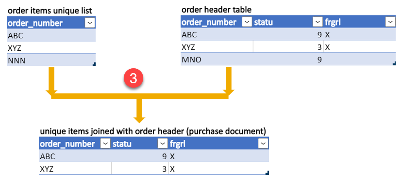
Figure 26: Step 3 - semi join of order items and order header
On this result the calculation will then be executed (see Step 4 - Fig. 27). Which means that in our example the order NNN and MNO won’t be part of our so-called purchase document as no matching record exists either in the items or in the header table. The SQL “SELECT * FROM A WHERE A.key IN (SELECT B.key from B)” would be the equivalent SQL expression.

Figure 27: Step 3 and step 4 - calculation for purchase documents in HEX Plan
In the final step 5 (Fig. 28) after the semi join the result from step 2 (applied filter) will be joined (via LEFT OUTER) with the result of step 4 (calculation).

Figure 28: Step 5 in HEX Plan
In the result (Fig. 28) now you can see that only for the order items ABC and XYZ the calculation gives a valid value. The calculation for order item NNN was not executed (MNO was removed by the filter on material) and that’s why NULL has to be shown due to the LEFT OUTER JOIN.
It’s a great new feature and performance improvement in HEX made available in the latest release of SAP HANA 2 which can be leveraged in different scenarios automatically without any changes to the model or application. However, it is still beneficial to remove the not null preserving pattern from your application model since this kind of transformation explained here requires two joins instead of one. E.g., in situations where no selective filter is applied the better choice would be to do the calculation on all items to avoid the additional semi join. Whether the semi join is used or not is decided by the optimizer based on estimated query costs and this of course increases the complexity of the query compilation, which in turn makes it harder to find a good execution plan and therefore increases compile times which may increases the risk that a sub-optimal execution plan is chosen.
- SAP Managed Tags:
- ABAP Development,
- SAP HANA,
- SAP S/4HANA
Labels:
1 Comment
You must be a registered user to add a comment. If you've already registered, sign in. Otherwise, register and sign in.
Labels in this area
-
Artificial Intelligence (AI)
1 -
Business Trends
363 -
Business Trends
24 -
Customer COE Basics and Fundamentals
1 -
Digital Transformation with Cloud ERP (DT)
1 -
Event Information
461 -
Event Information
24 -
Expert Insights
114 -
Expert Insights
164 -
General
1 -
Governance and Organization
1 -
Introduction
1 -
Life at SAP
415 -
Life at SAP
2 -
Product Updates
4,684 -
Product Updates
237 -
Roadmap and Strategy
1 -
Technology Updates
1,500 -
Technology Updates
89
Related Content
- Migrating data from SAP ECC to SAP S4/HANA with the migration cockpit in Enterprise Resource Planning Blogs by Members
- Enhancing Performance in SAP Web Applications: Strategies and Best Practices in Enterprise Resource Planning Blogs by Members
- What is the "standard" in Fit-to-Standard? in Enterprise Resource Planning Blogs by SAP
- Top 10+1 productivity boosting features that excite the business users of SAP S/4 Hana Sales in Enterprise Resource Planning Blogs by Members
- Streamline Your Journey to the Cloud with the RISE with SAP Methodology in Enterprise Resource Planning Blogs by SAP
Top kudoed authors
| User | Count |
|---|---|
| 12 | |
| 11 | |
| 7 | |
| 5 | |
| 5 | |
| 4 | |
| 4 | |
| 4 | |
| 3 | |
| 3 |