
- SAP Community
- Products and Technology
- Spend Management
- Spend Management Blogs by SAP
- Ariba Analytics using SAP Analytics Cloud, Data In...
Spend Management Blogs by SAP
Stay current on SAP Ariba for direct and indirect spend, SAP Fieldglass for workforce management, and SAP Concur for travel and expense with blog posts by SAP.
Turn on suggestions
Auto-suggest helps you quickly narrow down your search results by suggesting possible matches as you type.
Showing results for
Product and Topic Expert
Options
- Subscribe to RSS Feed
- Mark as New
- Mark as Read
- Bookmark
- Subscribe
- Printer Friendly Page
- Report Inappropriate Content
09-09-2022
10:31 AM
This is Part Two of a blog series on Ariba Analytics using SAP Analytics Cloud, Data Intelligence Cloud and HANA DocStore. If you would like to start with Part One, please click here
SAP Analytics Cloud makes it easy for businesses to understand their data through its stories, dashboards and analytical applications. Our worked example is using SAP Ariba Data to create an SAC Story that lets you know how much spend has been approved within Ariba Requisitions created in the last thirty days
In Part One of our blog series we discussed how we can retrieve data from SAP Ariba's APIs using SAP Data Intelligence Cloud. We stored this data as JSON Documents in the SAP HANA Document Store
In this blog post, we're going to build SQL and Calculation Views on top of our JSON Document Collection
In the third and final blog post we'll consume that Calculation View in SAP Analytics Cloud as a Live Data Model, which will provide the data to our SAP Analytics Cloud Story
As we discussed in our last blog post, objects within HANA usually have both a design-time and runtime artifact. Design-time artifacts are useful because they fully describe the object and can be deployed consistently across multiple HDI Containers or even HANA instances
Our JSON Document Collection has already been created, and is already storing our Ariba JSON Documents. From here, it's time to model our other artifacts
JSON Documents are useful in a variety of situations where you don't have strict, predefined schemas. When we retrieve our data from the Ariba APIs, we may retrieve data that doesn't map cleanly to a table schema (for example, data that is nested). Putting this data in the HANA DocStore Collection allows us to store the complete document, ensuring nothing is lost
In order for us to use this data for analytics, we'll need to map it to some sort of schema. We can create a logical schema on top of our Collection using a SQL View. This allows us to access a predefined subset of our data for analytics while leaving the full data untouched in our Collection
We'll create the SQL View in Business Application Studio
SQL Views use the following format:
If you're familiar with SQL, you may recognise this as the same syntax that you would use to create a standard SQL View, just missing the word "CREATE"
The SQL View doesn't duplicate any data, just provides a schema that we can use to access the underlying data
Our data in JSON Documents are Key-Value pairs
To retrieve the value "Complete", we would SELECT "Status"
JSON Documents may also have nested data
To retrieve the value "3728754507", we would SELECT "Content"."ItemId", with the full stop marking nested keys
Our example will use the following SQL View:
The fields we're using are only a fraction of the fields available in the Documents within our Collection - if we want to customize the scenario later, there are plenty more to choose from
We want to make sure this SQL View is deployed and ready for use, so click on the Deploy rocket
While we're in Business Application Studio, we're going to create our Calculation View. This Calculation View is what we'll be consuming in SAP Analytics Cloud
As before, we're using View->Find Command then Create SAP HANA Database Artifact
Business Application Studio has an inbuilt editor for Calculation Views, which we'll use to create ours
Now that our SQL View is available as a Data Source, we want to make sure its columns end up in our Calculation View
Because this is a Calculation View of type Cube (rather than Dimension), we'll need to make sure it includes at least one Measure
The columns in our SQL View all have the default data type NVARCHAR(5000). If we try to mark this column as a Measure directly, it will treat it as a string - giving us the Aggregation options COUNT, MIN and MAX
We want to treat this column as the number it is - as a workaround, we'll need to create a Calculated Column
A Calculated Column is an output column that we create within the Calculation View itself. Rather than being persisted, the values are calculated at runtime based on the result of an expression
For our example, we're using a very simple expression. First, we have to make our way to the Expression Editor
Next we're going to give our Calculated Column a name and data type. Because the granularity of our example is the Requisition-level and not the item-level, the decimal points won't meaningfully change the results. Given that, we're going to use the Integer data type
The Expression Editor is where we'll define how the column is calculated. Select our AmountInReportingCurrency Column
Our Created Column will take the value of AmountInReportingCurrency and convert it to an Integer
Now we want to validate the syntax of our Expression
We have one last thing to do inside our Calculation View - we want to filter the data to only include Approved Requisitions. If we want to use the Value Help to set our Filter, we'll need to Deploy the Calculation View
Before we Deploy our Calculation View, we want to make sure that we're only sending our integer Calculated Column and not the string version. To do this, we go the Semantics Node
All of the Columns we need, including our new Calculated Column are available within the Calculation View. Now we're ready to Deploy it one last time
Now that we've finished deploying our Design-time artifacts, we'll have the corresponding Runtime artifacts inside of our HDI Container. We can check these by going to SAP HANA Database Explorer from within Business Application Studio
In the Database Explorer, we want to first check on our SQL View
We can see all of the Columns in our created SQL View. If we want to check out some of the data returned by our SQL View, we can click on Open Data
Next it's time to check on our Calculation View
Database Explorer will open our Calculation View for Analysis. We're going to do our analysis in SAP Analytics Cloud, so for now we just want to verify the Raw Data
During this blog post we've built a SQL View and Calculation View on top of our HANA DocStore Collection. We've also made sure that our Calculation View only contains Approved Requisitions
In the third and final blog post we'll consume our Calculation View as a Live Data Model before visualizing it in an SAP Analytics Cloud Story. We'll also schedule the Data Intelligence Pipeline we created in our first blog post so that the data in our HANA DocStore Collection is updated on a regular basis automatically
SAP HANA Cloud | SQL Views
SAP HANA Cloud | Calculation Views
SAP HANA Cloud | SAP HANA Database Modeling Guide for SAP Business Application Studio
Business Application Studio | What is SAP Business Application Studio?
Business Application Studio | SAP Business Application Studio Overview by elizabeth.gutt (~ 5 minutes viewing time)
This blog series has had a lot of input from my colleagues – any errors are mine not theirs. In particular, thanks go to the Cross Product Management – SAP HANA Database & Analytics team, Antonio Maradiaga, Bengt Mertens, Andrei Tipoe, Melanie de Wit and Shabana Samsudheen
Note: While I am an employee of SAP, any views/thoughts are my own, and do not necessarily reflect those of my employer
Recap
SAP Analytics Cloud makes it easy for businesses to understand their data through its stories, dashboards and analytical applications. Our worked example is using SAP Ariba Data to create an SAC Story that lets you know how much spend has been approved within Ariba Requisitions created in the last thirty days

A simple SAC Story tracking Approved Requisitions
In Part One of our blog series we discussed how we can retrieve data from SAP Ariba's APIs using SAP Data Intelligence Cloud. We stored this data as JSON Documents in the SAP HANA Document Store
In this blog post, we're going to build SQL and Calculation Views on top of our JSON Document Collection
In the third and final blog post we'll consume that Calculation View in SAP Analytics Cloud as a Live Data Model, which will provide the data to our SAP Analytics Cloud Story

Viewing our HANA DocStore Collection data in an SAP Analytics Cloud Story
Design-Time Artifacts in Business Application Studio
As we discussed in our last blog post, objects within HANA usually have both a design-time and runtime artifact. Design-time artifacts are useful because they fully describe the object and can be deployed consistently across multiple HDI Containers or even HANA instances

When we deploy our design-time artifacts, they will be created as runtime artifacts inside our HDI Container
Our JSON Document Collection has already been created, and is already storing our Ariba JSON Documents. From here, it's time to model our other artifacts
Creating our SQL View
JSON Documents are useful in a variety of situations where you don't have strict, predefined schemas. When we retrieve our data from the Ariba APIs, we may retrieve data that doesn't map cleanly to a table schema (for example, data that is nested). Putting this data in the HANA DocStore Collection allows us to store the complete document, ensuring nothing is lost
In order for us to use this data for analytics, we'll need to map it to some sort of schema. We can create a logical schema on top of our Collection using a SQL View. This allows us to access a predefined subset of our data for analytics while leaving the full data untouched in our Collection
We'll create the SQL View in Business Application Studio

Click on View, then Find Command or press Ctrl+Shift+P

Use Find Command to find Create SAP HANA Database Artifact, then click on it

Select SQL View as the artifact type, and enter the artifact name then click on Create
SQL Views use the following format:
VIEW "aribaRequisitionSQLView"

AS SELECT "UniqueName", "Name", [...]

FROM "aribaRequisition"
If you're familiar with SQL, you may recognise this as the same syntax that you would use to create a standard SQL View, just missing the word "CREATE"
The SQL View doesn't duplicate any data, just provides a schema that we can use to access the underlying data
Our data in JSON Documents are Key-Value pairs
"Status":"Complete"To retrieve the value "Complete", we would SELECT "Status"
JSON Documents may also have nested data
"Content":{"ItemId":"3728754507"}To retrieve the value "3728754507", we would SELECT "Content"."ItemId", with the full stop marking nested keys
Our example will use the following SQL View:
VIEW "aribaRequisitionSQLView"

AS SELECT "UniqueName", "Name",

"TotalCost"."AmountInReportingCurrency" AS "AmountInReportingCurrency",

"ReportingCurrency"."UniqueName" AS "ReportingCurrency",

"ApprovedState", "Preparer"."UniqueName" AS "Preparer",

"Requester"."UniqueName" AS "Requester", "StatusString",

"CreateDate", "SubmitDate", "ApprovedDate", "LastModified",

"ProcurementUnit"."UniqueName" AS "ProcurementUnit"

FROM "aribaRequisition"
The fields we're using are only a fraction of the fields available in the Documents within our Collection - if we want to customize the scenario later, there are plenty more to choose from
We want to make sure this SQL View is deployed and ready for use, so click on the Deploy rocket
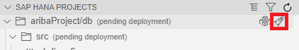
We can deploy our SQL View under SAP HANA Projects on the left
Creating our Calculation View
While we're in Business Application Studio, we're going to create our Calculation View. This Calculation View is what we'll be consuming in SAP Analytics Cloud
As before, we're using View->Find Command then Create SAP HANA Database Artifact

Choose Calculation View, enter a Name then click on Create
Business Application Studio has an inbuilt editor for Calculation Views, which we'll use to create ours

Click on Aggregation, then click the Plus symbol

Search for our SQL View, select it, then click Finish
Now that our SQL View is available as a Data Source, we want to make sure its columns end up in our Calculation View

Click on Aggregation, then click on Expand Details

Click on our SQL View on the left then drag and drop to Output Columns on the right

Our SQL view columns will now be available in our Calculation View
Because this is a Calculation View of type Cube (rather than Dimension), we'll need to make sure it includes at least one Measure
The columns in our SQL View all have the default data type NVARCHAR(5000). If we try to mark this column as a Measure directly, it will treat it as a string - giving us the Aggregation options COUNT, MIN and MAX
We want to treat this column as the number it is - as a workaround, we'll need to create a Calculated Column
Creating our Calculated Column
A Calculated Column is an output column that we create within the Calculation View itself. Rather than being persisted, the values are calculated at runtime based on the result of an expression
For our example, we're using a very simple expression. First, we have to make our way to the Expression Editor

Click on Calculated Columns

Create a Calculated Column using the Plus symbol, then Calculated Column

Click on the Arrow
Next we're going to give our Calculated Column a name and data type. Because the granularity of our example is the Requisition-level and not the item-level, the decimal points won't meaningfully change the results. Given that, we're going to use the Integer data type
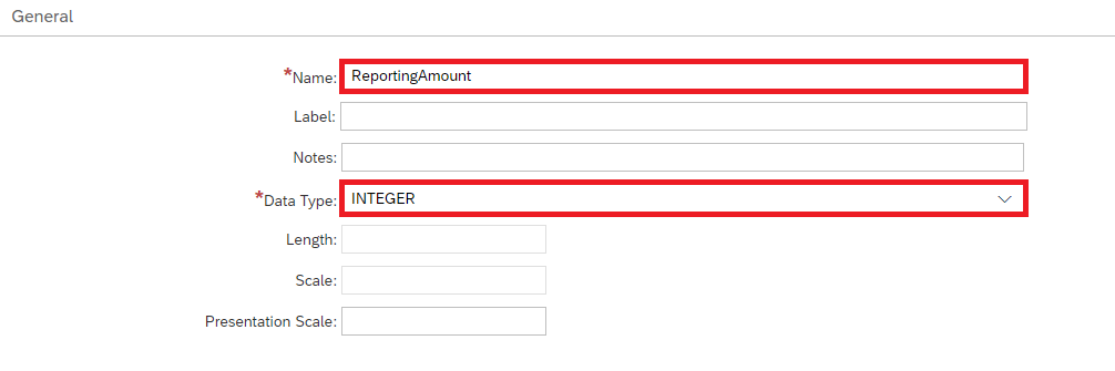
Give the Calculated Column a Name, and choose the Data Type Integer

Choose Measure as the Column Type

Click on Expression Editor
The Expression Editor is where we'll define how the column is calculated. Select our AmountInReportingCurrency Column
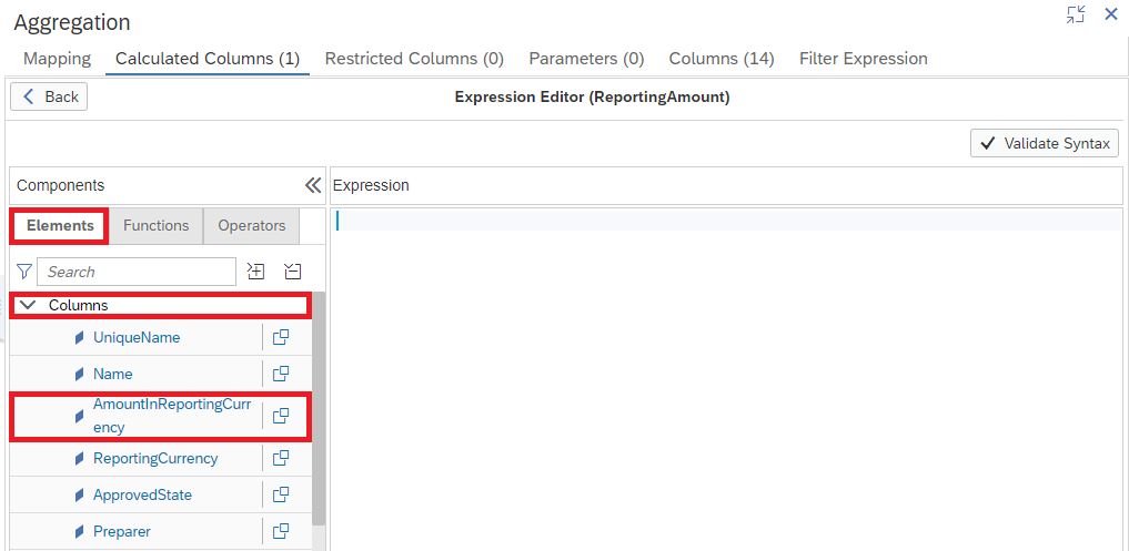
Select our Column from the left

Our Column is in the Expression
Our Created Column will take the value of AmountInReportingCurrency and convert it to an Integer
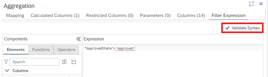
Now we want to validate the syntax of our Expression

Click on Validate Syntax

Our Expression is valid
We have one last thing to do inside our Calculation View - we want to filter the data to only include Approved Requisitions. If we want to use the Value Help to set our Filter, we'll need to Deploy the Calculation View

Deploy our Calculation View

Click on Filter Expression

Click on ApprovedState under Columns
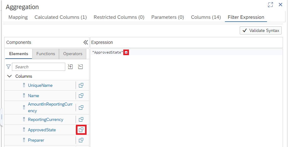
Add an Equals Sign (=) then click on the Value Help

Select Approved then click OK
Now we can check the syntax of our Filter
Click on Validate Syntax

Our Filter is valid
Before we Deploy our Calculation View, we want to make sure that we're only sending our integer Calculated Column and not the string version. To do this, we go the Semantics Node

Click on Semantics, then Columns
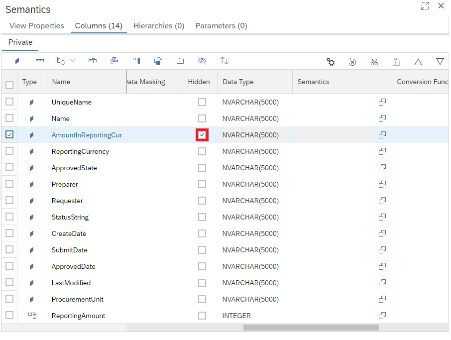
Check Hidden for our AmountInReportingCurrency Column to exclude it from our Calculation View
All of the Columns we need, including our new Calculated Column are available within the Calculation View. Now we're ready to Deploy it one last time

Once again, click on the Deploy Rocket under SAP HANA Projects
Checking our Runtime Artifacts
Now that we've finished deploying our Design-time artifacts, we'll have the corresponding Runtime artifacts inside of our HDI Container. We can check these by going to SAP HANA Database Explorer from within Business Application Studio

Click on Open HDI Container on the left under SAP HANA Projects
In the Database Explorer, we want to first check on our SQL View

Click Views on the left, then click on our SQL View

Our SQL View
We can see all of the Columns in our created SQL View. If we want to check out some of the data returned by our SQL View, we can click on Open Data

Click on Open Data

Data from our SQL View is displayed
Next it's time to check on our Calculation View

Click Column Views on the left, then click on our Calculation View

Our Calculation View

Click on Open Data
Database Explorer will open our Calculation View for Analysis. We're going to do our analysis in SAP Analytics Cloud, so for now we just want to verify the Raw Data

Click on Raw Data

Data from our Calculation View is displayed
Wrap-Up
During this blog post we've built a SQL View and Calculation View on top of our HANA DocStore Collection. We've also made sure that our Calculation View only contains Approved Requisitions
In the third and final blog post we'll consume our Calculation View as a Live Data Model before visualizing it in an SAP Analytics Cloud Story. We'll also schedule the Data Intelligence Pipeline we created in our first blog post so that the data in our HANA DocStore Collection is updated on a regular basis automatically
Other Resources
SAP HANA Cloud | SQL Views
SAP HANA Cloud | Calculation Views
SAP HANA Cloud | SAP HANA Database Modeling Guide for SAP Business Application Studio
Business Application Studio | What is SAP Business Application Studio?
Business Application Studio | SAP Business Application Studio Overview by elizabeth.gutt (~ 5 minutes viewing time)
Special Thanks
This blog series has had a lot of input from my colleagues – any errors are mine not theirs. In particular, thanks go to the Cross Product Management – SAP HANA Database & Analytics team, Antonio Maradiaga, Bengt Mertens, Andrei Tipoe, Melanie de Wit and Shabana Samsudheen
Note: While I am an employee of SAP, any views/thoughts are my own, and do not necessarily reflect those of my employer
Labels:
You must be a registered user to add a comment. If you've already registered, sign in. Otherwise, register and sign in.
Labels in this area
-
Business Trends
113 -
Business Trends
12 -
Event Information
44 -
Event Information
3 -
Expert Insights
18 -
Expert Insights
25 -
Life at SAP
32 -
Product Updates
253 -
Product Updates
27 -
Technology Updates
82 -
Technology Updates
14
Related Content
- Mastering Procurement Analytics: Essential Strategies and Safeguards for Success in Spend Management Blogs by SAP
- The Procurement Monthly - March 2024 in Spend Management Blogs by SAP
- Navigating the Data-Driven World of Procurement Analytics: The Roadmap to Achieving Best-In-Class St in Spend Management Blogs by SAP
- Boosting Business Success with Procurement Analytics: A Journey Paved with Numbers in Spend Management Blogs by SAP
- SAP Analytics for Cloud and SAP Ariba - Data Connections in Spend Management Q&A
Top kudoed authors
| User | Count |
|---|---|
| 2 | |
| 1 | |
| 1 | |
| 1 | |
| 1 | |
| 1 | |
| 1 | |
| 1 | |
| 1 |