
- SAP Community
- Groups
- Interest Groups
- Application Development
- Blog Posts
- Safeguard Performance of ABAP CDS Views – Part 2 H...
Application Development Blog Posts
Learn and share on deeper, cross technology development topics such as integration and connectivity, automation, cloud extensibility, developing at scale, and security.
Turn on suggestions
Auto-suggest helps you quickly narrow down your search results by suggesting possible matches as you type.
Showing results for
former_member18
Active Participant
Options
- Subscribe to RSS Feed
- Mark as New
- Mark as Read
- Bookmark
- Subscribe
- Printer Friendly Page
- Report Inappropriate Content
11-28-2018
5:39 PM
In this blog post I describe how the HANA optimizer creates an execution plan from your SQL statement, how this plan wanders into the plan cache and what you should consider when analyzing the SQL statement from HANA studio. Since my main interest is the performance of CDS views, I will concentrate on the resource and runtime aspects.
Here is the agenda of the blog series:
In the previous blog post we have seen that the SQL statement that is created when a CDS view is accessed in ABAP code might become quite complex. On top of the ‘static’ complexity of the view itself, additional tables or views might be joined when associations are followed, or when the view has assigned DCLs (Data Control Language objects, that is authority checks).
For HANA to be able to respond to a database request, it needs an execution plan for the SQL statement, that is a kind of recipe that describes how to retrieve the data and prepare the output. This recipe is not in the SQL statement itself, since SQL is a declarative language: it just describes ‘what’ to be processed, not the ‘how’. There is no specification, whether a certain join should be processed before or after doing some aggregation, nor whether the database should apply a nested-loop join, a hash join, or a semi join to get to the result. In fact, the ‘how’ is left to the SQL processor, which does, based on the rules of relational algebra and with the help of database table statistics, come up with an execution plan to process the SQL statement.

During the process of plan creation, the information given in the SQL string is used by the SQL processor to create multiple plans that are evaluated to find the best (or at least a good) execution plan. Ideally, join reordering is possible between all joins of the SQL statement, and also other operators like filters or aggregations can be ‘moved around’ in the plan variants.
The SQL processor is quite smart in finding its way through the 'logical plan forest', and it's amazing that even for SQL statements with many dozens of tables a plan can be created that allows efficient data access. But still, the SQL optimizer cannot work wonders:
In the end it is the quality of the data model and the way the data is accessed that determine – at least when it comes to many millions of table entries – the execution runtime of a SQL statement.
Besides the SQL statement, the SQL optimizer considers several other factors that influence the plan creation and the effectiveness of the resulting plan, for example:
The picture below shows two screen shots from HANA PlanViz. The executed statement was the same for both plans, but the system and the data constellation were different. One finds that the resulting plans are totally different; for example, the critical path containing the slowest operators (red circles) changed its position. That is why complex statements must be tested with production-like data to achieve relevant results.

As we have seen, to determine the execution plan for a complex SQL statement thousands of different plan variants are evaluated. The screen shot below shows the SQL Plan Cache for SQL statements having a high plan preparation time (column TOTAL_PREPARATION_TIME). The values are given in µs, so these statements took many seconds for plan preparation.

This preparation time depends on the complexity of the SQL statement, and it adds up to the total execution time of a statement – so it should not be neglected! Below we will see that this issue is mitigated by the HANA plan cache.
To avoid surprises with erratic or slow performance of CDS views, you should
For long running analytical queries it can be OK to spend some time and memory for plan creation and statement compilation in every execution. This is not possible for SQL statements executed in transactional processes where response times in the millisecond range are required. Here the preparation time would probably exceed the execution time. That is why SAP HANA stores optimized SQL statements in a plan cache. It associates the SQL string (plus some additional info) of a query with the compiled query execution plan. Identical statements need not to be parsed, and plans not be recompiled every time, but only after plan invalidations / evictions (see end of blog).
But what are identical SQL statements? If you want to investigate some performance issue with the HANA PlanViz tool, you are of course interested to obtain a plan that is relevant for your performance problem. As shown in the picture below, even a small comment in one of two otherwise identical SQL statements can lead to different execution plans that might - as in this example from HANA studio - have different runtimes:

This effect is not critical for SQL statements created by some framework, since they will always have the same format. It's a bit more relevant for hand-written ABAP SQL, since also a different order of the fields in the WHERE-clause leads to different plans. For SQL statements in ABAP there is the recommendation to specify the fields in the WHERE-clause in the same order that the fields have in the accessed dictionary object (table or SQL view).
Another important factor for statement identity are the parameters of an SQL statement (CDS view parameters and parameters in WHERE-clause, GROUP BY, ORDER BY, ...). If every parameter set of an SQL statement would lead to an own plan cache entry, the cache would soon be filled with tons of structural-identical statements. To avoid this, statements coming from ABAP are send to the database with bind variables for most of the parameter values (shown as ‘?’ in the SQL statement in ST05 SQL Trace). Only if ABAP recognizes that a parameter value is a constant, it will be passed as literal value to the database.
In the picture below, in the ABAP code snippet on the left side the parameter value @LV_product_name for parameter PRODUCTNAME might vary in every execution of the statement. Together with the implicitly added client field, this parameter value shows up as '?' in the SQL statement in ST05 (right side). The value for SUPPLIERNAME on the other hand is hardcoded as 'ASAP' and is passed as literal value to the database. In the SQL Trace Record this value is displayed as literal.
The statement displayed in the SQL Trace Record is the one that is stored in the plan cache (see screen shot from HANA plan cache at bottom of picture).

Often there is an SQL statement, for example from ST05 trace, that one wants to (re-)execute from HANA studio to see its current runtime behavior or to create a HANA PlanViz plan. In most cases, you want to trigger the same statement as the ABAP execution did, to employ the same cached plan.
For passing statement parameters to HANA, in HANA studio you can explicitly choose between the two possibilities of passing a parameter value as literal or passing it as bind variable.
The SQL optimizer will handle these two variants differently:
Note that only the second variant reflects what is done from ABAP! Only when using bind variables and literals in HANA studio the same way as in the ABAP execution, the same plan will be employed.
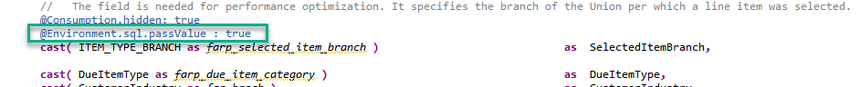
As mentioned, using host variables for execution from ABAP (leading to using bind variables in HANA) is a means for ‘resource-friendliness’ as it saves space in the plan cache that would otherwise be flooded with plans of structure-identical statements. This is weighting the resource plan cache in favor of a potentially better optimized plan for a statement using the literal values. Still, in some cases it can be reasonable to allow the SQL optimizer to do its job with some more information and explicitly pass parameters as literals. This can be accomplished in the CDS view by using the field annotation @Environment.sql.passValue: true.
This option should be restricted to fields with only a few different possible values, and its benefit for the statement execution time should be verified.
Plan cache entries are invalidated when involved data structures are changed. Also, the HANA join engine may force a recompilation if the amount of data in one of the underlying data sources changes drastically (more than doubles or halves). On HANA, you will find the invalidation reason for some plan in system view M_SQL_PLAN_CACHE in column LAST_INVALIDATION_REASON.
When the plan cache is full, and a newly created plan needs to be cached, the cache detects candidates for eviction by scanning the list of the least recently used entries and removes plans that are not currently in-use by an active statement.
Remember the following effects of the plan cache that can influence the analysis of SQL statements and CDS views:
Here is the agenda of the blog series:
- Part 1 – CDS View Complexity
- Part 2 – HANA SQL Optimizer and Plan Cache – this blog
- Part 3 – Rules for Good Performance of CDS Views
- Part 4 – Data Modelling
- Part x – maybe more … your ideas or questions
In the previous blog post we have seen that the SQL statement that is created when a CDS view is accessed in ABAP code might become quite complex. On top of the ‘static’ complexity of the view itself, additional tables or views might be joined when associations are followed, or when the view has assigned DCLs (Data Control Language objects, that is authority checks).
SQL Optimizer / Processor
For HANA to be able to respond to a database request, it needs an execution plan for the SQL statement, that is a kind of recipe that describes how to retrieve the data and prepare the output. This recipe is not in the SQL statement itself, since SQL is a declarative language: it just describes ‘what’ to be processed, not the ‘how’. There is no specification, whether a certain join should be processed before or after doing some aggregation, nor whether the database should apply a nested-loop join, a hash join, or a semi join to get to the result. In fact, the ‘how’ is left to the SQL processor, which does, based on the rules of relational algebra and with the help of database table statistics, come up with an execution plan to process the SQL statement.
During the process of plan creation, the information given in the SQL string is used by the SQL processor to create multiple plans that are evaluated to find the best (or at least a good) execution plan. Ideally, join reordering is possible between all joins of the SQL statement, and also other operators like filters or aggregations can be ‘moved around’ in the plan variants.
Note that the SQL string processed by the SQL processor does not retain any information on the CDS entities that were involved to create the SQL statement - neither does the resulting execution plan. It is therefore sometimes difficult to trace back a performance problem, which has been identified in the HANA PlanViz tool, to the corresponding CDS view. For an effective performance analysis, a good knowledge of the underlying data model (that is, of the involved CDS entities) is essential.
Through the Forest
The SQL processor is quite smart in finding its way through the 'logical plan forest', and it's amazing that even for SQL statements with many dozens of tables a plan can be created that allows efficient data access. But still, the SQL optimizer cannot work wonders:
- The SQL processor must always guarantee correct results; therefore, it must obey to the semantics of the SQL query. This leads to a situation, where optimizations that are desirable from a high-level perspective (e.g. removal of joins, or loop optimizations by aggregating data before executing further calculations or joins) are not always possible.
Example: aggregation push-down
SUM( ROUND( convert_currency( VALUE, EUR ) , 2 ) )  "is not equivalent to

ROUND( convert_currency( SUM( VALUE ), EUR ), 2 )
In the first case, the currency conversion has to be executed for every line item before the rounding and the summation can be executed. In the second case, only the summed-up value needs to be converted. Since these cases have different semantics (and might return different results), the SQL processor may not switch the order of the operators. - The number of possible plan variants strongly rises (steeper than the factorial) with the number of underlying tables (see here for a deep dive into join ordering). Since the SQL processor needs to make decisions in a short time frame, it will only evaluate a limited number (some thousands) of possible plan variants. The chosen plan might therefore be not the theoretical / global ‘best’ plan, if – as a rule of thumb – an SQL statement joins more than 5 tables.
- Due to the many different potential plan variants for complex SQL statements, one cannot be sure that after a re-compilation of a plan, the same plan will be selected as in a previous plan determination. In the worst case this can lead to an erratic runtime behavior, with a statement running slow that before has been executed quite fast.
- The SQL processor cannot fix gruesome data models (for example by adding secondary indexes or by refusing calculations on critical fields) nor awkward accesses to data (e.g. reading all data without any filter).
Example: a CDS view has a calculated key field; here the key field is concatenated from two other fields
define view cdsTest as select from dbtab

{ key CONCAT( fld2, fld3 ) AS concatKey,

... }
If such a calculated field is used as filter in a WHERE-clause, a calculation (here: concatenation) on millions of entries might be necessary before the filter can be applied. When used in a join condition, a calculated field may hinder the push-down of a filter to one of the joined branches.
In the end it is the quality of the data model and the way the data is accessed that determine – at least when it comes to many millions of table entries – the execution runtime of a SQL statement.
Influence of Data
Besides the SQL statement, the SQL optimizer considers several other factors that influence the plan creation and the effectiveness of the resulting plan, for example:
- Data statistics – a plan based on an optimization done in a test system, with only sparely filled tables, can differ fundamentally from a plan for the same SQL statement executed in a production system with 100’s of millions of table entries (see picture below)
- Indices – though HANA can often do without secondary indices, there are situations where they help, see SAP note.
- Physical schema design, for example partitioning of tables or indices
- Plan creation also depends on the implementation of the query optimizer and the HANA engines. After a HANA upgrade a certain portion of SQL statements will result in different execution plans.
The picture below shows two screen shots from HANA PlanViz. The executed statement was the same for both plans, but the system and the data constellation were different. One finds that the resulting plans are totally different; for example, the critical path containing the slowest operators (red circles) changed its position. That is why complex statements must be tested with production-like data to achieve relevant results.
Preparation Time
As we have seen, to determine the execution plan for a complex SQL statement thousands of different plan variants are evaluated. The screen shot below shows the SQL Plan Cache for SQL statements having a high plan preparation time (column TOTAL_PREPARATION_TIME). The values are given in µs, so these statements took many seconds for plan preparation.
This preparation time depends on the complexity of the SQL statement, and it adds up to the total execution time of a statement – so it should not be neglected! Below we will see that this issue is mitigated by the HANA plan cache.
Recommendations (1)
To avoid surprises with erratic or slow performance of CDS views, you should
- Keep CDS views as simple as possible, only as complex as needed to achieve the target of the business case. As mentioned above, the SQL optimizer might not be able to identify the ‘best’ plan for a SQL statement, if complexity gets too high. Also, execution plans and execution times for complex SQL statements might change after re-creation of plans.
- Thoroughly test important SQL statements with production-like data (i.e. both amount of data and data distribution should be realistic) before using them productively. Trace and analyze single critical SQL statements with ST05 (Performance Trace) and HANA PlanViz.
- After an HANA upgrade, or when the amount of data in underlying tables has changed drastically, control the execution of business-critical SQL statements.
- Monitor overall SQL performance with HANA Plan Cache or SQLM (SQL monitoring tool on ABAP server).
- Follow instructions in note 1794297 to detect tables that might benefit from secondary indices
HANA Plan Cache
For long running analytical queries it can be OK to spend some time and memory for plan creation and statement compilation in every execution. This is not possible for SQL statements executed in transactional processes where response times in the millisecond range are required. Here the preparation time would probably exceed the execution time. That is why SAP HANA stores optimized SQL statements in a plan cache. It associates the SQL string (plus some additional info) of a query with the compiled query execution plan. Identical statements need not to be parsed, and plans not be recompiled every time, but only after plan invalidations / evictions (see end of blog).
Identical Statements
But what are identical SQL statements? If you want to investigate some performance issue with the HANA PlanViz tool, you are of course interested to obtain a plan that is relevant for your performance problem. As shown in the picture below, even a small comment in one of two otherwise identical SQL statements can lead to different execution plans that might - as in this example from HANA studio - have different runtimes:
This effect is not critical for SQL statements created by some framework, since they will always have the same format. It's a bit more relevant for hand-written ABAP SQL, since also a different order of the fields in the WHERE-clause leads to different plans. For SQL statements in ABAP there is the recommendation to specify the fields in the WHERE-clause in the same order that the fields have in the accessed dictionary object (table or SQL view).
Parameters
Another important factor for statement identity are the parameters of an SQL statement (CDS view parameters and parameters in WHERE-clause, GROUP BY, ORDER BY, ...). If every parameter set of an SQL statement would lead to an own plan cache entry, the cache would soon be filled with tons of structural-identical statements. To avoid this, statements coming from ABAP are send to the database with bind variables for most of the parameter values (shown as ‘?’ in the SQL statement in ST05 SQL Trace). Only if ABAP recognizes that a parameter value is a constant, it will be passed as literal value to the database.
In the picture below, in the ABAP code snippet on the left side the parameter value @LV_product_name for parameter PRODUCTNAME might vary in every execution of the statement. Together with the implicitly added client field, this parameter value shows up as '?' in the SQL statement in ST05 (right side). The value for SUPPLIERNAME on the other hand is hardcoded as 'ASAP' and is passed as literal value to the database. In the SQL Trace Record this value is displayed as literal.
The statement displayed in the SQL Trace Record is the one that is stored in the plan cache (see screen shot from HANA plan cache at bottom of picture).
When preparing a plan for an SQL statement with parameters for the very first time, the SQL optimizer creates an initial plan based on the statement with place holders, and then immediately a second query compilation is triggered based on the bind variables of this first execution (parameter aware optimization). This allows a more accurate size estimation and creates a more efficient plan.
Execution from HANA studio
Often there is an SQL statement, for example from ST05 trace, that one wants to (re-)execute from HANA studio to see its current runtime behavior or to create a HANA PlanViz plan. In most cases, you want to trigger the same statement as the ABAP execution did, to employ the same cached plan.
For passing statement parameters to HANA, in HANA studio you can explicitly choose between the two possibilities of passing a parameter value as literal or passing it as bind variable.
- Passing values for MANDT and PRODUCTNAME as literal values:

- Passing values for MANDT and PRODUCTNAME as bind variables. On execution, you will have to specify the bind variables on the follow-up screen:

The SQL optimizer will handle these two variants differently:
- In the first case, a plan will be generated that is optimized exactly for the specified literal values. If the plan already exists in plan cache, it will be a 100% fit for the parameter values.
- In the second case, a plan will be created using bind variables and ‘parameter aware optimization’. If the plan already exists in plan cache, the parameter aware optimization might have been previously executed with a different set of bind variables.
Note that only the second variant reflects what is done from ABAP! Only when using bind variables and literals in HANA studio the same way as in the ABAP execution, the same plan will be employed.
Optimization Using Literals
As mentioned, using host variables for execution from ABAP (leading to using bind variables in HANA) is a means for ‘resource-friendliness’ as it saves space in the plan cache that would otherwise be flooded with plans of structure-identical statements. This is weighting the resource plan cache in favor of a potentially better optimized plan for a statement using the literal values. Still, in some cases it can be reasonable to allow the SQL optimizer to do its job with some more information and explicitly pass parameters as literals. This can be accomplished in the CDS view by using the field annotation @Environment.sql.passValue: true.
This option should be restricted to fields with only a few different possible values, and its benefit for the statement execution time should be verified.
Plan Cache Invalidation and Eviction
Plan cache entries are invalidated when involved data structures are changed. Also, the HANA join engine may force a recompilation if the amount of data in one of the underlying data sources changes drastically (more than doubles or halves). On HANA, you will find the invalidation reason for some plan in system view M_SQL_PLAN_CACHE in column LAST_INVALIDATION_REASON.
When the plan cache is full, and a newly created plan needs to be cached, the cache detects candidates for eviction by scanning the list of the least recently used entries and removes plans that are not currently in-use by an active statement.
Recommendations (2)
Remember the following effects of the plan cache that can influence the analysis of SQL statements and CDS views:
- Execution of SQL statements from ABAP using host variables for CDS view parameters or parameter values in the WHERE-clause will lead to execution plans based on bind variables
- To obtain reliable runtime results and reproducible HANA PlanViz plans in HANA studio, consider whether bind variables or literals should be used
- Small variations of the SQL statement in HANA studio lead to the creation of different execution plans
- In ABAP try to implement your SQL statements 'cache-friendly'. This means, the structure of statements accessing the same table or CDS view should always be the same, for example stating the fields of the WHERE-clause in the same order that the fields have in the accessed dictionary object.
- SAP Managed Tags:
- ABAP Development
17 Comments
You must be a registered user to add a comment. If you've already registered, sign in. Otherwise, register and sign in.
Labels in this area
-
A Dynamic Memory Allocation Tool
1 -
ABAP
8 -
abap cds
1 -
ABAP CDS Views
14 -
ABAP class
1 -
ABAP Cloud
1 -
ABAP Development
4 -
ABAP in Eclipse
1 -
ABAP Keyword Documentation
2 -
ABAP OOABAP
2 -
ABAP Programming
1 -
abap technical
1 -
ABAP test cockpit
7 -
ABAP test cokpit
1 -
ADT
1 -
Advanced Event Mesh
1 -
AEM
1 -
AI
1 -
API and Integration
1 -
APIs
8 -
APIs ABAP
1 -
App Dev and Integration
1 -
Application Development
2 -
application job
1 -
archivelinks
1 -
Automation
4 -
BTP
1 -
CAP
1 -
CAPM
1 -
Career Development
3 -
CL_GUI_FRONTEND_SERVICES
1 -
CL_SALV_TABLE
1 -
Cloud Extensibility
8 -
Cloud Native
7 -
Cloud Platform Integration
1 -
CloudEvents
2 -
CMIS
1 -
Connection
1 -
container
1 -
Debugging
2 -
Developer extensibility
1 -
Developing at Scale
4 -
DMS
1 -
dynamic logpoints
1 -
Eclipse ADT ABAP Development Tools
1 -
EDA
1 -
Event Mesh
1 -
Expert
1 -
Field Symbols in ABAP
1 -
Fiori
1 -
Fiori App Extension
1 -
Forms & Templates
1 -
IBM watsonx
1 -
Integration & Connectivity
10 -
JavaScripts used by Adobe Forms
1 -
joule
1 -
NodeJS
1 -
ODATA
3 -
OOABAP
3 -
Outbound queue
1 -
Product Updates
1 -
Programming Models
13 -
RFC
1 -
RFFOEDI1
1 -
SAP BAS
1 -
SAP BTP
1 -
SAP Build
1 -
SAP Build apps
1 -
SAP Build CodeJam
1 -
SAP CodeTalk
1 -
SAP Odata
1 -
SAP UI5
1 -
SAP UI5 Custom Library
1 -
SAPEnhancements
1 -
SapMachine
1 -
security
3 -
text editor
1 -
Tools
16 -
User Experience
5
Top kudoed authors
| User | Count |
|---|---|
| 6 | |
| 5 | |
| 3 | |
| 3 | |
| 2 | |
| 2 | |
| 2 | |
| 1 | |
| 1 | |
| 1 |