
- SAP Community
- Products and Technology
- Technology
- Technology Blogs by SAP
- Google Vertex AI triggering calculations / ML in S...
Technology Blogs by SAP
Learn how to extend and personalize SAP applications. Follow the SAP technology blog for insights into SAP BTP, ABAP, SAP Analytics Cloud, SAP HANA, and more.
Turn on suggestions
Auto-suggest helps you quickly narrow down your search results by suggesting possible matches as you type.
Showing results for
Product and Topic Expert
Options
- Subscribe to RSS Feed
- Mark as New
- Mark as Read
- Bookmark
- Subscribe
- Printer Friendly Page
- Report Inappropriate Content
01-09-2023
1:50 PM
If Google Vertex AI is part of your landscape, you might enjoy the option to use your familiar Google Cloud environment to trigger data processing in your SAP Data Warehouse Cloud / SAP HANA Cloud systems.
Connect from Vertex AI (or other Google components) to the data in SAP Data Warehouse Cloud / SAP HANA Cloud and carry out data explorations, preparations, calculations, and Machine Learning. The data remains in place, thereby avoiding data movement and data duplication. Save your outcomes as semantic views or physical tables in the SAP system. And if needed, you can still extract the data into Google Cloud for further processing. However, you might not need to move all granular records, just the aggregated / prepared / filtered / predicted data that you require. Google Cloud can then further process the data and outcomes can still be written back back to SAP Data Warehouse Cloud / SAP HANA Cloud.
If you would like to stay instead within the SAP Business Technology Platform, you have the familiar choices to deploy your Python / R code with SAP Data Intelligence, CloudFoundry and Kyma. Apart from Google Vertex AI you can can also use virtually any Python or R environment. Either way, SAP’s Python package hana_ml and R package hana.ml.r make it easy to trigger such an advanced analysis from Python or R on the data held in SAP Data Warehouse Cloud / SAP HANA Cloud.
Should this use case and blog be somewhat familiar to you, then you have probably already seen a related blog, which explains the same scenario with Azure Machine Learning, Databricks or Dataiku as front end.
Let’s use a time series forecast as sandboxing example for triggering Machine Learning calculations in SAP Data Warehouse Cloud from Google Vertex AI. You will create a Jupyter notebook in Vertex AI to sandbox the scenario. Explore the data stored in SAP Data Warehouse Cloud, aggregate it and create a time series forecast on the aggregates. All triggered from Vertex AI, executed in SAP Data Warehouse Cloud.
In this scenario we are assuming that you are working with SAP Data Warehouse Cloud. However, an implementation with SAP HANA Cloud would be very similar:
You also need to have access to Google Vertex AI.
Begin by creating a new project on the Google Cloud Console and enable these APIs:
In the Vertex AI Workbench create a user-managed notebook. You have to use such a "user-managed notebook", as I understand that the alternative of "managed notebooks" do not provide external IP addresses. An external IP address is required so that Vertex AI can communicate with SAP Data Warehouse Cloud.
JupyterLab opens up. Then click on "Python 3" in the notebooks section on the right to create the notebook we will execute our code in.
In the Notebook that has opened, run this line to install the hana_ml Python library, which allows Python to trigger activities in SAP Data Warehouse Cloud (or SAP HANA Cloud or SAP HANA on-premise). Essentially, the hana_ml library translates the instructions made in Python to SQL code. When scripting in Python, you can obtain the SQL code, but you don't need to. The library shapely is installed, since some of the hana_ml functionality (that is not used in this example though) requires it as dependency.
With the hana_ml library installed, you can establish a connection to the SAP Data Warehouse Cloud. Just enter your database user’s details as a quick test (see prerequisites above). This code should result with the output “True”, to confirm that the connection was created.
Should this fail, you might still need to add the IP address of the JupyterLab environment to the “IP Allowlist” in SAP Data Warehouse Cloud. If you are not sure about your external IP address, you can find it out with this quick test. Your Google Cloud Platform architect will be able to advise on specifying a permanent IP address or range for your setup.
Using the SAP Data Warehouse Cloud password in the code was a quick test. To keep the logon credentials more secure, you can store the password in Google's Secret Manager. See the final section of this blog for the detailed steps.
In your own projects you might be working with data that is already in SAP Data Warehouse Cloud. To follow this blog’s example, upload some test data into the system for us to work with. First load the Power consumption of Tetouan city Data Set from the UCI Machine Learning Repository into a pandas DataFrame. (Salam, A., & El Hibaoui, A. (2018, December). Comparison of Machine Learning Algorithms for the Power Consumption Prediction:-Case Study of Tetouan city“. In 2018 6th International Renewable and Sustainable Energy Conference (IRSEC) (pp. 1-5). IEEE).
The data shows the power consumption of the Moroccan city in 10-minute intervals for the year 2017. We will use the data to create a time series forecast.
Use the hana_ml library and the connection that you have already established, to load this data into SAP Data Warehouse Cloud. The table and the appropriate columns will be created automatically.
Create a hana_ml DataFrame, which points to the data that remains in SAP Data Warehouse Cloud. We will be using this object extensively. Its collect() method can return the data as pandas DataFrame. To have a peek at the data, just select 5 rows.
You can check on the column types.
Have SAP Data Warehouse Cloud calculate some statistics about the data content.
The above distribution statistics were all calculated in SAP Data Warehouse Cloud. Only the results were transferred to your notebook. You can see the SELECT statement that was created by the describe() method.
You can also request further calculations on the data, or use ready-made exploratory plots. Have SAP Data Warehouse Cloud calculate a correlation matrix on the granular data. As you would expect, there is for instance a fair positive correlation between temperature and power consumption.
Now plot part of the data’s time series. Download the records of the last 7 days and plot them locally. The calculation 6 * 24 * 7 specifies how many most recent rows we are interested in. The data is in 10-minute intervals, so 6 gets a full hour. Multiplied by 24 to get a day, multiplied by 7 to get one week. The power consumption clearly has a strong daily pattern.
For further analysis add a DATE and MONTH column. These columns are added logically to the hana_ml DataFrame. The original table remains unchanged. Not data gets duplicated.
With the MONTH column, we can now create a boxplot that shows how consumption changes through the year. August has the highest median consumption.
Let’s get ready for a daily forecast. Have SAP Data Warehouse Cloud aggregate the 10-minute intervals to daily aggregates. Save the aggregation logic as view in the SAP Data Warehouse Cloud and show a few of the aggregated rows. The view could come in handy if you want to create the forecast within Google Cloud on aggregated data. You would have reduced the amount of data that needs to travel.
Plot the daily consumption of the last 3 weeks.
SAP Data Warehouse Cloud has an Automated ML framework built-in as well as 100+ individual algorithms. The hana_ml library’s documentation has all the details. For our time series forecast we choose to use an AdditiveModelForecast, which is an implementation of the Prophet algorithm, and train a model.
To create predictions, you just need to specify for which dates predictions should be produced. Use the historic data (on which the model was trained) to dynamically obtain a pandas DataFrame, which lists the future 21 dates, for which we want to create a prediction.
Bring this data through the hana_ml library as temporary table to SAP Data Warehouse Cloud.
Use the temporary table as input for the prediction.
With the prediction now available as hana_ml DataFrame, you are free to use the predictions as required by your use case. Download the predictions for instance into a pandas DataFrame and have them plotted. The weekly pattern is nicely represented.
Or look at the predictions, still from Vertex AI. Here with the predicted columns renamed before the display.
Or save the predictions as table to SAP Data Warehouse Cloud, where SAP Analytics Cloud, or another tool of your choice could pick up the predictions to share them with a broader user base.
You have used Vertex AI to explore data in SAP Data Warehouse Cloud, to prepare the data, to create a forecast and to share the predictions to SAP Analytics Cloud. No data got duplicated along the way, thereby reducing architectural and governmental complexity. This logic can be further automated and scheduled of course by Vertex AI for productive use. However, you can also choose from range of alternative to schedule the code with Google Cloud Platform. See for example this option with Google Cloud Functions.
In the above example the password of the SAP Data Warehouse Cloud user was hardcoded in clear text in Python. That might be ok for a quick test, but you will really want to keep the password more secure. This optional section explains how to keep the password safe with Google's Secret Manager.
To be able to access the secret from the Jupyter Notebook, go in the Google Cloud Dashboard menu to "IAM and admin", find your "developer.gserviceaccount.com" and add the role "Secret Manager" → "Secret Accessor".
In your notebook you then need to install the google-cloud-secret-manager library.
And you can now retrieve the password from the Secret Manager. Change the name parameter to the resource ID that you copied earlier.
A combination of Cloud Functions and Google Scheduler seems a quick and easy option to have the code executed regularly. This example assumes that you have stored the password of the SAP Data Warehouse Cloud user in the Secret Manager.
First create a Cloud Function:
Enter the code for a Python runtime:
For the requirements.txt:
Deploy the Cloud Function so that a REST-API is created to trigger the code.
And you can use the Cloud Scheduler to automatically call that REST-API, thereby scheduling the creation of new forecasts.
You got to know how to use Python in Google Vertex AI and Google Cloud Functions to trigger calculations and Machine Learning in SAP Data Warehouse Cloud. Hence you can keep the data where it is, or download / upload the data to and from Vertex AI as required.
Connect from Vertex AI (or other Google components) to the data in SAP Data Warehouse Cloud / SAP HANA Cloud and carry out data explorations, preparations, calculations, and Machine Learning. The data remains in place, thereby avoiding data movement and data duplication. Save your outcomes as semantic views or physical tables in the SAP system. And if needed, you can still extract the data into Google Cloud for further processing. However, you might not need to move all granular records, just the aggregated / prepared / filtered / predicted data that you require. Google Cloud can then further process the data and outcomes can still be written back back to SAP Data Warehouse Cloud / SAP HANA Cloud.
If you would like to stay instead within the SAP Business Technology Platform, you have the familiar choices to deploy your Python / R code with SAP Data Intelligence, CloudFoundry and Kyma. Apart from Google Vertex AI you can can also use virtually any Python or R environment. Either way, SAP’s Python package hana_ml and R package hana.ml.r make it easy to trigger such an advanced analysis from Python or R on the data held in SAP Data Warehouse Cloud / SAP HANA Cloud.
Should this use case and blog be somewhat familiar to you, then you have probably already seen a related blog, which explains the same scenario with Azure Machine Learning, Databricks or Dataiku as front end.

Let’s use a time series forecast as sandboxing example for triggering Machine Learning calculations in SAP Data Warehouse Cloud from Google Vertex AI. You will create a Jupyter notebook in Vertex AI to sandbox the scenario. Explore the data stored in SAP Data Warehouse Cloud, aggregate it and create a time series forecast on the aggregates. All triggered from Vertex AI, executed in SAP Data Warehouse Cloud.
Prerequisites
In this scenario we are assuming that you are working with SAP Data Warehouse Cloud. However, an implementation with SAP HANA Cloud would be very similar:
- You need access to a SAP Data Warehouse Cloud system with three virtual CPUs (free trial is not sufficient)
- The script server must be activated, see the documentation
- Create a Database User in your SAP Data Warehouse Cloud space, with the options “Enable Automated Predictive Library and Predictive Analysis Library”, “Enable Read Access” and “Enable Write Access” selected, see the documentation
- To trigger the Machine Learning in SAP Data Warehouse Cloud, you need that user’s password and the system’s host name, see this tutorial
You also need to have access to Google Vertex AI.
Google Cloud Project
Begin by creating a new project on the Google Cloud Console and enable these APIs:
- Vertex AI API
- Notebooks API for scripting Python in a Jupyter Notebook
- Secret Manager API [optional] to securely store the user name and password for accessing SAP Data Warehouse Cloud
Google Cloud Vertex AI
In the Vertex AI Workbench create a user-managed notebook. You have to use such a "user-managed notebook", as I understand that the alternative of "managed notebooks" do not provide external IP addresses. An external IP address is required so that Vertex AI can communicate with SAP Data Warehouse Cloud.

As environment for the notebook you can select "Python 3" and the smallest possible Machine type, ie n1-standard-1. After all, the calculations will mostly happen in SAP Data Warehouse Cloud. Hence a small type is sufficient. For this blog^s example you can keep all other default settings, which includes the activated option to "enable external IP address

JupyterLab opens up. Then click on "Python 3" in the notebooks section on the right to create the notebook we will execute our code in.
Connection to SAP Data Warehouse Cloud
In the Notebook that has opened, run this line to install the hana_ml Python library, which allows Python to trigger activities in SAP Data Warehouse Cloud (or SAP HANA Cloud or SAP HANA on-premise). Essentially, the hana_ml library translates the instructions made in Python to SQL code. When scripting in Python, you can obtain the SQL code, but you don't need to. The library shapely is installed, since some of the hana_ml functionality (that is not used in this example though) requires it as dependency.
%pip install hana-ml==2.15.22122300

%pip install shapely
With the hana_ml library installed, you can establish a connection to the SAP Data Warehouse Cloud. Just enter your database user’s details as a quick test (see prerequisites above). This code should result with the output “True”, to confirm that the connection was created.
import hana_ml.dataframe as dataframe

conn = dataframe.ConnectionContext(address='[YOURDBUSERSHOSTNAME]',

                                   port=443,

                                   user='[YOURDBUSER]',

                                   password='[YOURDBUSERSPASSWORD]')

conn.connection.isconnected()
Should this fail, you might still need to add the IP address of the JupyterLab environment to the “IP Allowlist” in SAP Data Warehouse Cloud. If you are not sure about your external IP address, you can find it out with this quick test. Your Google Cloud Platform architect will be able to advise on specifying a permanent IP address or range for your setup.
from urllib.request import urlopen

import re as r

def getIP():

    d = str(urlopen('http://checkip.dyndns.com/').read())

    return r.compile(r'Address: (\d+\.\d+\.\d+\.\d+)').search(d).group(1)

print(getIP())
Using the SAP Data Warehouse Cloud password in the code was a quick test. To keep the logon credentials more secure, you can store the password in Google's Secret Manager. See the final section of this blog for the detailed steps.
Time series forecasting
In your own projects you might be working with data that is already in SAP Data Warehouse Cloud. To follow this blog’s example, upload some test data into the system for us to work with. First load the Power consumption of Tetouan city Data Set from the UCI Machine Learning Repository into a pandas DataFrame. (Salam, A., & El Hibaoui, A. (2018, December). Comparison of Machine Learning Algorithms for the Power Consumption Prediction:-Case Study of Tetouan city“. In 2018 6th International Renewable and Sustainable Energy Conference (IRSEC) (pp. 1-5). IEEE).
The data shows the power consumption of the Moroccan city in 10-minute intervals for the year 2017. We will use the data to create a time series forecast.
import pandas as pd

df_data = pd.read_csv('https://archive.ics.uci.edu/ml/machine-learning-databases/00616/Tetuan%20City%20power%20consumption.csv')

df_data.columns = map(str.upper, df_data.columns)

df_data.columns = df_data.columns.str.replace(' ', '_')

df_data.DATETIME = pd.to_datetime(df_data.DATETIME)
Use the hana_ml library and the connection that you have already established, to load this data into SAP Data Warehouse Cloud. The table and the appropriate columns will be created automatically.
import hana_ml.dataframe as dataframe

df_remote = dataframe.create_dataframe_from_pandas(connection_context=conn,

                                                   pandas_df=df_data,

                                                   table_name='POWERCONSUMPTION',

                                                   force=True,

                                                   replace=False)
Create a hana_ml DataFrame, which points to the data that remains in SAP Data Warehouse Cloud. We will be using this object extensively. Its collect() method can return the data as pandas DataFrame. To have a peek at the data, just select 5 rows.
df_remote = conn.table('POWERCONSUMPTION')

df_remote.head(5).collect()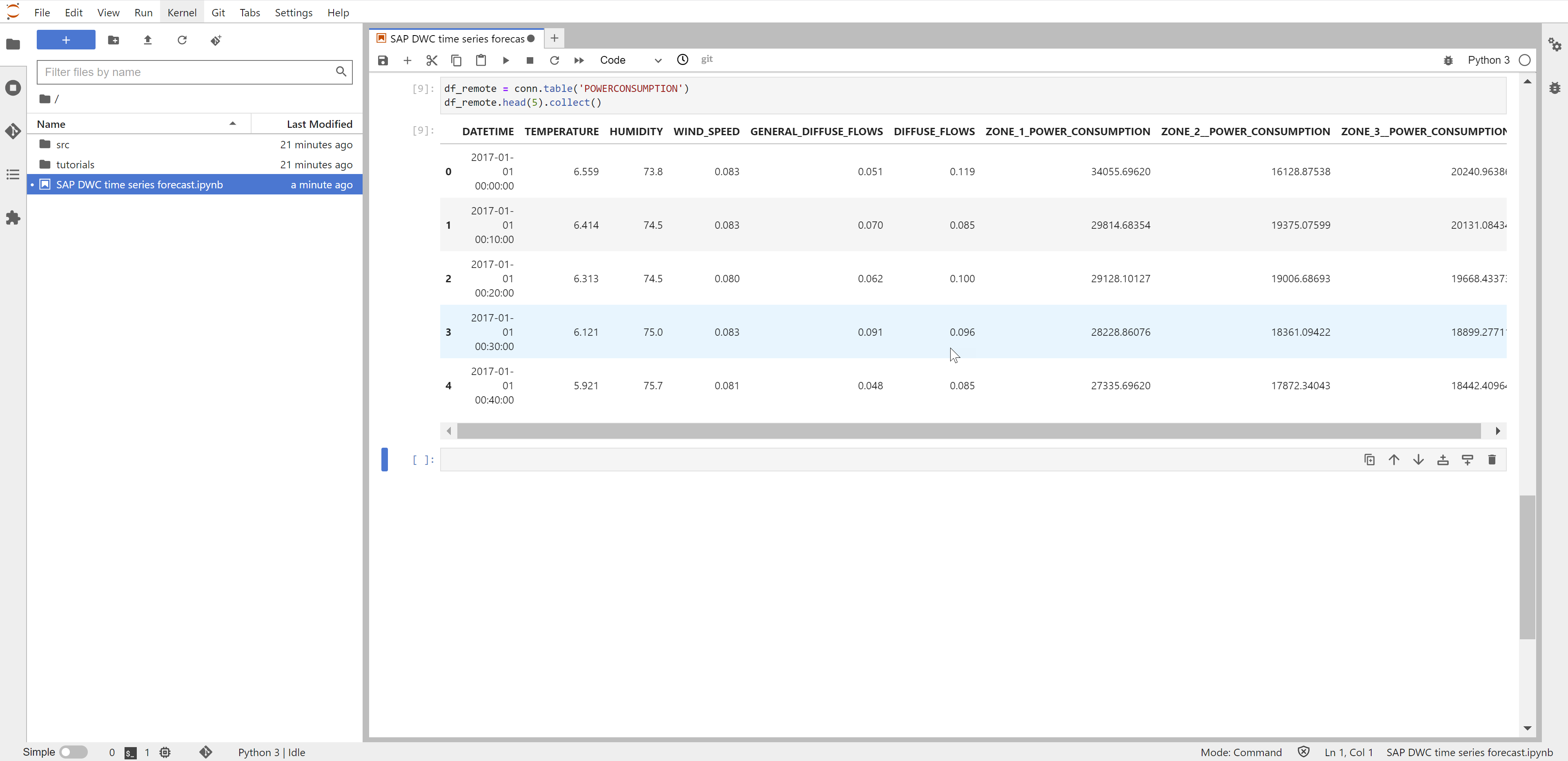
You can check on the column types.
df_remote.dtypes()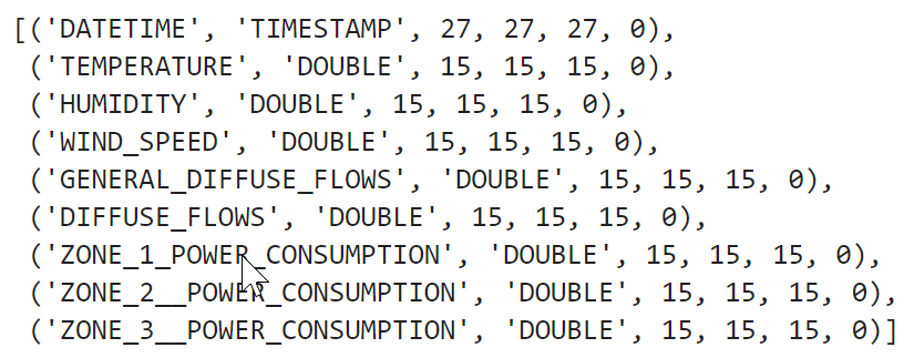
Have SAP Data Warehouse Cloud calculate some statistics about the data content.
df_remote.describe().collect()
The above distribution statistics were all calculated in SAP Data Warehouse Cloud. Only the results were transferred to your notebook. You can see the SELECT statement that was created by the describe() method.
print(df_remote.describe().select_statement)
You can also request further calculations on the data, or use ready-made exploratory plots. Have SAP Data Warehouse Cloud calculate a correlation matrix on the granular data. As you would expect, there is for instance a fair positive correlation between temperature and power consumption.
import matplotlib.pyplot as plt

from hana_ml.visualizers.eda import EDAVisualizer

f = plt.figure()

ax1 = f.add_subplot(111) # 111 refers to 1x1 grid, 1st subplot

eda = EDAVisualizer(ax1)

ax, corr_data = eda.correlation_plot(data=df_remote, cmap='coolwarm')
Now plot part of the data’s time series. Download the records of the last 7 days and plot them locally. The calculation 6 * 24 * 7 specifies how many most recent rows we are interested in. The data is in 10-minute intervals, so 6 gets a full hour. Multiplied by 24 to get a day, multiplied by 7 to get one week. The power consumption clearly has a strong daily pattern.
df_data = df_remote.tail(n=6*24*7, ref_col='DATETIME').collect()

df_data.drop('DATETIME', axis=1).plot(subplots=True,

                                    figsize=(10, 14));
For further analysis add a DATE and MONTH column. These columns are added logically to the hana_ml DataFrame. The original table remains unchanged. Not data gets duplicated.
df_remote = conn.table('POWERCONSUMPTION')

df_remote = df_remote.select('*', ('TO_DATE(DATETIME)', 'DATE'))

df_remote = df_remote.select('*', ('LEFT(DATE, 7)', 'MONTH'))

df_remote.head(5).collect()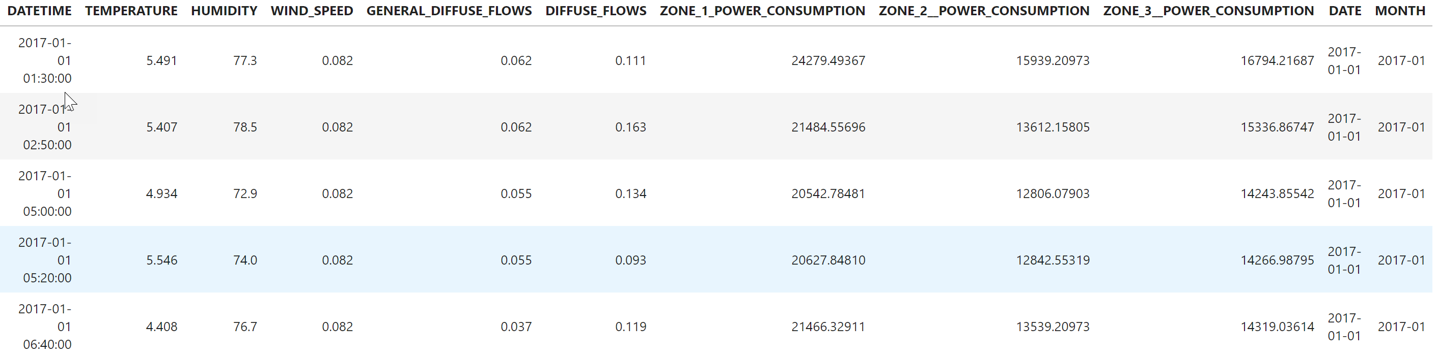
With the MONTH column, we can now create a boxplot that shows how consumption changes through the year. August has the highest median consumption.
import matplotlib.pyplot as plt

from hana_ml.visualizers.eda import EDAVisualizer

f = plt.figure()

ax1 = f.add_subplot(111) # 111 refers to 1x1 grid, 1st subplot

eda = EDAVisualizer(ax1)

ax, cont = eda.box_plot(data=df_remote,

                        column='ZONE_1_POWER_CONSUMPTION', groupby='MONTH', outliers=True)

ax.legend(bbox_to_anchor=(1, 1));
Let’s get ready for a daily forecast. Have SAP Data Warehouse Cloud aggregate the 10-minute intervals to daily aggregates. Save the aggregation logic as view in the SAP Data Warehouse Cloud and show a few of the aggregated rows. The view could come in handy if you want to create the forecast within Google Cloud on aggregated data. You would have reduced the amount of data that needs to travel.
df_remote_daily = df_remote.agg([('sum', 'ZONE_1_POWER_CONSUMPTION', 'ZONE_1_POWER_CONSUMPTION_SUM')], group_by='DATE')

df_remote_daily.save('V_POWERCONSUMPTION_DAILY', force=True)

df_remote_daily.head(5).collect()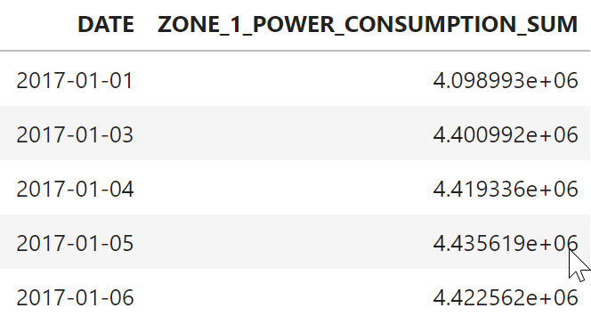
Plot the daily consumption of the last 3 weeks.
df_data = df_remote_daily.tail(n=21, ref_col='DATE').collect()


import matplotlib.pyplot as plt

from matplotlib.pyplot import figure

figure(figsize=(12, 5))

plt.plot(df_data['DATE'], df_data['ZONE_1_POWER_CONSUMPTION_SUM'])

plt.xticks(rotation=45);
SAP Data Warehouse Cloud has an Automated ML framework built-in as well as 100+ individual algorithms. The hana_ml library’s documentation has all the details. For our time series forecast we choose to use an AdditiveModelForecast, which is an implementation of the Prophet algorithm, and train a model.
from hana_ml.algorithms.pal.tsa.additive_model_forecast import AdditiveModelForecast

amf = AdditiveModelForecast(growth='linear')

amf.fit(data=df_remote_daily.select('DATE', 'ZONE_1_POWER_CONSUMPTION_SUM'))
To create predictions, you just need to specify for which dates predictions should be produced. Use the historic data (on which the model was trained) to dynamically obtain a pandas DataFrame, which lists the future 21 dates, for which we want to create a prediction.
import pandas as pd

strLastDate = str( df_remote_daily.select('DATE').max())

df_topredict = pd.date_range(strLastDate, periods=1 + 21, freq="D", closed='right').to_frame()

df_topredict.columns = ['DATE']

df_topredict['DUMMY'] = 0

df_topredict
Bring this data through the hana_ml library as temporary table to SAP Data Warehouse Cloud.
import hana_ml.dataframe as dataframe

df_rem_topredict = dataframe.create_dataframe_from_pandas(connection_context=conn,

                                                   pandas_df=df_topredict,

                                                   table_name='#TOPREDICTDAILY',

                                                   force=True,

                                                   replace=False)
Use the temporary table as input for the prediction.
df_rem_predicted = amf.predict(data=df_rem_topredict)With the prediction now available as hana_ml DataFrame, you are free to use the predictions as required by your use case. Download the predictions for instance into a pandas DataFrame and have them plotted. The weekly pattern is nicely represented.
df_data = df_rem_predicted.collect()


from matplotlib import pyplot as plt

figure(figsize=(12, 5))

plt.plot(df_data['DATE'], df_data['YHAT'])

plt.fill_between(df_data['DATE'],df_data['YHAT_LOWER'], df_data['YHAT_UPPER'], alpha=.3)

plt.xticks(rotation=45);
Or look at the predictions, still from Vertex AI. Here with the predicted columns renamed before the display.
df_rem_predicted = df_rem_predicted.rename_columns(['DATE', 'PREDICTION', 'PREDICTION_LOWER', 'PREDICTION_UPPER'])

df_rem_predicted.collect()
Or save the predictions as table to SAP Data Warehouse Cloud, where SAP Analytics Cloud, or another tool of your choice could pick up the predictions to share them with a broader user base.
df_rem_predicted.save('POWERCONSUMPTION_21DAYPRED', force=True)
You have used Vertex AI to explore data in SAP Data Warehouse Cloud, to prepare the data, to create a forecast and to share the predictions to SAP Analytics Cloud. No data got duplicated along the way, thereby reducing architectural and governmental complexity. This logic can be further automated and scheduled of course by Vertex AI for productive use. However, you can also choose from range of alternative to schedule the code with Google Cloud Platform. See for example this option with Google Cloud Functions.
Store password in Secret Manager
In the above example the password of the SAP Data Warehouse Cloud user was hardcoded in clear text in Python. That might be ok for a quick test, but you will really want to keep the password more secure. This optional section explains how to keep the password safe with Google's Secret Manager.
If you have already enabled the Secret Manager API, you can find the Secret Manager through the Google Cloud Dashboard menu on the left hand side in the "Security" section. Create a new secret and store the password as secret value. Once created, copy the resource ID from the Actions drop-down.

To be able to access the secret from the Jupyter Notebook, go in the Google Cloud Dashboard menu to "IAM and admin", find your "developer.gserviceaccount.com" and add the role "Secret Manager" → "Secret Accessor".
In your notebook you then need to install the google-cloud-secret-manager library.
%pip install google-cloud-secret-managerAnd you can now retrieve the password from the Secret Manager. Change the name parameter to the resource ID that you copied earlier.
from google.cloud import secretmanager

client = secretmanager.SecretManagerServiceClient()

name = 'projects/965005017854/secrets/DWC_password/versions/1'

response = client.access_secret_version(request={"name": name})

DWC_password = response.payload.data.decode("UTF-8")

import hana_ml.dataframe as dataframe

conn = dataframe.ConnectionContext(address='[YOURDBUSERSHOSTNAME]',

                                   port=443,

                                   user='[YOURDBUSER]',

                                   password=DWC_password)

conn.connection.isconnected()
Google Cloud Functions
A combination of Cloud Functions and Google Scheduler seems a quick and easy option to have the code executed regularly. This example assumes that you have stored the password of the SAP Data Warehouse Cloud user in the Secret Manager.
First create a Cloud Function:
- of trigger type HTTP, so that the execution can be triggered through a REST-API
- with an allocated memory of 256 MB (128 MB might not be sufficient)
- with a maximum timeout of 540 seconds (the default of 60 seconds might be too short for the forecast to complete in time)
- under a Runtime service account, that has the role "Secret Manager Secret Accessor".
Enter the code for a Python runtime:
def ts_forecast(request):

    """Responds to any HTTP request.

    Args:

        request (flask.Request): HTTP request object.

    Returns:

        The response text or any set of values that can be turned into a

        Response object using

        `make_response <http://flask.pocoo.org/docs/1.0/api/#flask.Flask.make_response>`.

    """

    request_json = request.get_json()

    if request.args and 'message' in request.args:

        return request.args.get('message')

    elif request_json and 'message' in request_json:

        return request_json['message']

    else:

      # Get SAP DWC password from Secret Manager

      from google.cloud import secretmanager

      client = secretmanager.SecretManagerServiceClient()

      name = 'projects/965005017854/secrets/DWC_password/versions/1'

      response = client.access_secret_version(request={"name": name})

      DWC_password = response.payload.data.decode("UTF-8")


      # Conntection to SAP DWC

      import hana_ml.dataframe as dataframe

      conn = dataframe.ConnectionContext(address='[YOURDBUSERSHOSTNAME]',

                                   port=443,

                                   user='[YOURDBUSER]',

                                   password=DWC_password)


      # Point to the view of the daily aggregates

      df_remote_daily = conn.table('V_POWERCONSUMPTION_DAILY')


      # Train the time series model

      from hana_ml.algorithms.pal.tsa.additive_model_forecast import AdditiveModelForecast

      amf = AdditiveModelForecast(growth='linear')

      amf.fit(data=df_remote_daily.select('DATE', 'ZONE_1_POWER_CONSUMPTION_SUM'))


      # Dates to predict

      import pandas as pd

      strLastDate = str(df_remote_daily.select('DATE').max())

      df_topredict = pd.date_range(strLastDate, periods=1 + 21, freq="D", closed='right').to_frame()

      df_topredict.columns = ['DATE']

      df_topredict['DUMMY'] = 0


      # Upload the dates that are to be predicted as temporary table

      df_rem_topredict = dataframe.create_dataframe_from_pandas(connection_context=conn,

                                                                pandas_df=df_topredict,

                                                                table_name='#TOPREDICTDAILY',

                                                                force=True,

                                                                replace=False)


      # Create the forecast

      df_rem_predicted = amf.predict(data=df_rem_topredict)


      # Save forecast as permanent table

      tableName = 'POWERCONSUMPTION_21DAYPRED_GCPCF'

      df_rem_predicted.save(tableName, force=True)


      # Success message

      return f'The forecasts have been saved to table {tableName}'
For the requirements.txt:
google-cloud-secret-manager

hana-ml==2.15.22122300

shapely
Deploy the Cloud Function so that a REST-API is created to trigger the code.

And you can use the Cloud Scheduler to automatically call that REST-API, thereby scheduling the creation of new forecasts.

Summary
You got to know how to use Python in Google Vertex AI and Google Cloud Functions to trigger calculations and Machine Learning in SAP Data Warehouse Cloud. Hence you can keep the data where it is, or download / upload the data to and from Vertex AI as required.
Labels:
You must be a registered user to add a comment. If you've already registered, sign in. Otherwise, register and sign in.
Labels in this area
-
ABAP CDS Views - CDC (Change Data Capture)
2 -
AI
1 -
Analyze Workload Data
1 -
BTP
1 -
Business and IT Integration
2 -
Business application stu
1 -
Business Technology Platform
1 -
Business Trends
1,661 -
Business Trends
88 -
CAP
1 -
cf
1 -
Cloud Foundry
1 -
Confluent
1 -
Customer COE Basics and Fundamentals
1 -
Customer COE Latest and Greatest
3 -
Customer Data Browser app
1 -
Data Analysis Tool
1 -
data migration
1 -
data transfer
1 -
Datasphere
2 -
Event Information
1,400 -
Event Information
65 -
Expert
1 -
Expert Insights
178 -
Expert Insights
280 -
General
1 -
Google cloud
1 -
Google Next'24
1 -
Kafka
1 -
Life at SAP
784 -
Life at SAP
11 -
Migrate your Data App
1 -
MTA
1 -
Network Performance Analysis
1 -
NodeJS
1 -
PDF
1 -
POC
1 -
Product Updates
4,577 -
Product Updates
330 -
Replication Flow
1 -
RisewithSAP
1 -
SAP BTP
1 -
SAP BTP Cloud Foundry
1 -
SAP Cloud ALM
1 -
SAP Cloud Application Programming Model
1 -
SAP Datasphere
2 -
SAP S4HANA Cloud
1 -
SAP S4HANA Migration Cockpit
1 -
Technology Updates
6,886 -
Technology Updates
408 -
Workload Fluctuations
1
Related Content
- New Machine Learning features in SAP HANA Cloud in Technology Blogs by SAP
- What’s New in SAP Analytics Cloud Release 2024.07 in Technology Blogs by SAP
- SAP Datasphere - Space, Data Integration, and Data Modeling Best Practices in Technology Blogs by SAP
- Porting Legacy Data Models in SAP Datasphere in Technology Blogs by SAP
- Recap — SAP Data Unleashed 2024 in Technology Blogs by Members
Top kudoed authors
| User | Count |
|---|---|
| 13 | |
| 10 | |
| 10 | |
| 9 | |
| 7 | |
| 6 | |
| 5 | |
| 5 | |
| 5 | |
| 4 |