
- SAP Community
- Products and Technology
- Technology
- Technology Blogs by SAP
- Street-level maps with openstreetmaps.org for Lumi...
Technology Blogs by SAP
Learn how to extend and personalize SAP applications. Follow the SAP technology blog for insights into SAP BTP, ABAP, SAP Analytics Cloud, SAP HANA, and more.
Turn on suggestions
Auto-suggest helps you quickly narrow down your search results by suggesting possible matches as you type.
Showing results for
Product and Topic Expert
Options
- Subscribe to RSS Feed
- Mark as New
- Mark as Read
- Bookmark
- Subscribe
- Printer Friendly Page
- Report Inappropriate Content
06-19-2015
9:14 PM
In previous articles I have discussed political maps of countries and topographical maps. One thing I noticed, though, when going through that is that there are limits to how much you can "zoom" into those maps, when based on Natural Earth shape files. So, I went looking for something else that could provide lower level of detail, and found that with openstreetmap.org.
OpenStreetMap is an open source map of the world that individual contributors put together based on their local knowledge as well as satellite imagery. I am a such a contributor myself. Much of the world is very well covered (especially Europe, it appears), going as detailed as individual buildings and even smaller elements. Other parts of the world can be somewhat less detailed, but if something is missing, it would be highly appreciated if you helped add it in!
So, in order to do an experiment to see how this worked practically, I decided to pick the SAP Walldorf campus. This is what that looks like in OpenStreetMap when on the "export" screen:
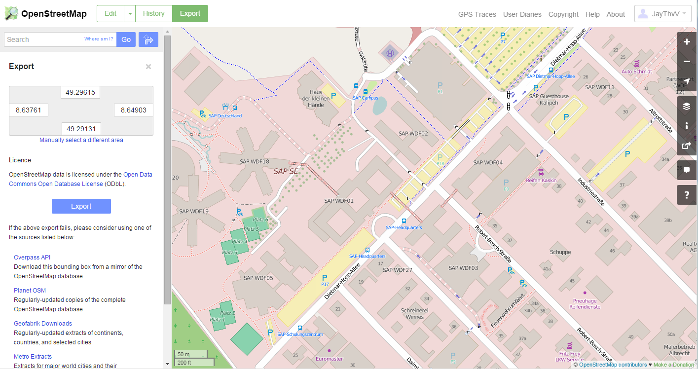
You can actually get a sense of the amount of detail that is included. This shows all buildings, but even bus routes, individual trees, bicycle parking, and even the tennis courts and volleyball field. I've been to the campus many times before, but wasn't even aware it had a helipad! But this will be more than satisfactory for my map experiment.
As I described before, I prefer to generate my own GeoJSON/topoJSON map files. OpenStreetMap allows you to export sections of the map as OSM files, which can be handled by ogr2ogr, a tool I discussed in previous articles. What you can see already on this screen underneath the "Export" title, is the viewing box with coordinates of what you're looking at, so this is even easier than getting your coordinates for the viewing box from Google Maps. OSM exports can very quickly become very large in size when you take larger areas, but there are services you can use (underneath the blue export button) to export such larger maps as a batch process. Don't even try to download the whole OSM worldmap as it runs over 1TB in size, and it is updated all the time...
The exported OSM file will be called map.osm, when exported directly from OpenStreetMap. The first thing to do is to extract points, lines, multilinestrings and multipolygons from it into separate shape files. You can try to do it directly in one go, but this gives some errors as there are some features not supported, and this avoids that issue. I have this in a make file, like this:
# make shape files from the OSM file
wdf-lines.shp: map.osm
ogr2ogr --config OSM_USE_CUSTOM_INDEXING NO -skipfailures -clipdst $(BOUNDS) -f "ESRI Shapefile" wdf-lines.shp map.osm -overwrite lines
wdf-points.shp: map.osm
ogr2ogr --config OSM_USE_CUSTOM_INDEXING NO -skipfailures -clipdst $(BOUNDS) -f "ESRI Shapefile" wdf-points.shp map.osm -overwrite points
wdf-multiline.shp: map.osm
ogr2ogr --config OSM_USE_CUSTOM_INDEXING NO -skipfailures -clipdst $(BOUNDS) -f "ESRI Shapefile" wdf-multiline.shp map.osm -overwrite multilinestrings
wdf-multipoly.shp: map.osm
ogr2ogr --config OSM_USE_CUSTOM_INDEXING NO -skipfailures -clipdst $(BOUNDS) -f "ESRI Shapefile" wdf-multipoly.shp map.osm -overwrite multipolygons
Note how I am again using the -clipdst option with saved coordinates in BOUNDS. This was described in a previous article, and even though the exported file should already be filtered, I found that if I didn't do this, I had a bit of extra space around the area I really wanted, so clipping like this helps get around that. I simply use the same coordinates that you saw in the export screenshot from OpenStreetMap. For the rest, just realize that the lines starting ogr2ogr are one line (even if they spill over into a second here.)
Next there are two steps you can take to figure out what is in each of these generated shape files. One way is to use the ogrinfo tool that allows you to look for specific properties in each of these files, including with a SQL-like syntax. Another way it to generate a GeoJSON file from these shape files (just run ogr2ogr with the -f GeoJSON option) so you can look at it in a human readable format. What also certainly helps it to take a look at the OpenStreetMap Map Features. Moreover, what I try to do is to make life as easy as possible for me in the D3.js JavaScript code, by doing as much filtering as possible within the map generation. Let's look at this example:
# landuse
landuse.json: wdf-multipoly.shp
ogr2ogr -f "GeoJSON" -where "landuse IS NOT NULL" landuse.json wdf-multipoly.shp
"Land use" in OpenStreetMap refers to multipolygon areas that can be of different kinds, like "residential", "commercial", "farmland", etc. What I am doing in this command line is simply create a separate landuse GeoJSON file containing anything in that wdf-multipoly shape file where the landuse property is not null, and make sure that the landuse property itself is present in the topojson command, so it is carried over into the resulting JSON file and we can use it during visualization:
wdf-sap.json: roads.json buildings.json parking.json landuse.json leisure.json streams.json
topojson --id-property name -p name,highway,landuse,leisure -o wdf-sap.json -- roads.json buildings.json parking.json landuse.json leisure.json streams.json
As you can see from the files listed in that command, I am also extracting roads, buildings, parking areas, leisure and streams in a similar way.
Now, here is what the entire JavaScript code is to draw all landuse areas into the map:
var landuse = topojson.feature(wdf, wdf.objects.landuse);
...
svg.selectAll(".landuse")
.data(landuse.features)
.enter().append("path")
.attr("class", "landuse")
.attr("type", function(d){ return d.properties.landuse; })
.attr("d", path);
That's it! I then use the "type" attribute with the name of the landuse item, to style that type of landuse with CSS:
.landuse[type="grass"]{
stroke: #0f0;
fill: #40FF40;
}
.landuse[type="commercial"]{
fill: #c0a0a0;
opacity: 0.5;
}
.landuse[type="farmland"]{
fill: #808000;
opacity: 0.5;
}
.landuse[type="recreation_ground"]{
fill: #80F000;
opacity: 0.5;
}
And that gets me the following result (with the SVG itself having a background-color of #d0e0d0):

If I was going to be real nit-picky, I would handle this slightly differently, as in this set the commercial is drawn last, and that then overlaps over the grass areas, making those a bit darker than I would like, but for this experiment I didn't bother.
Buildings and leisure are extracted in exactly the same way. I am styling all buildings the same, and leisure only is for the tennis court and volleyball fields, so I don't style those on type:

Parking areas are "amenities", and to make sure I pick up all, the line in my make file is like this:
# parking
parking.json: wdf-multipoly.shp
ogr2ogr -f "GeoJSON" -where "amenity IN ('parking', 'parking_space', 'bicycle_parking')" parking.json wdf-multipoly.shp
Roads are extracted from wdf-lines.shp , the converted OSM "lines" data, with the 'highway IS NOT NULL' where clause and styled again with CSS:
.roads[type="service"]{
stroke: #f8f8f8;
stroke-width: 3;
fill: none;
}
.roads[type="platform"]{
stroke: #f8f8f8;
stroke-width: 3;
fill: none;
}
.roads[type="residential"]{
stroke: #f8f8f8;
stroke-width: 4;
fill: none;
}
.roads[type="footway"]{
stroke: #A08080;
stroke-width: 1;
fill: none;
}
.roads[type="path"]{
stroke: #A08080;
stroke-width: 1;
fill: none;
}
.roads[type="track"]{
stroke: #806060;
stroke-width: 1;
fill: none;
}
.roads[type="cycleway"]{
stroke: #f8f8f8;
stroke-width: 2;
fill: none;
}
.roads[type="primary"]{
stroke: #f8f8f8;
stroke-width: 8;
fill: none;
}
.roads[type="primary_link"]{
stroke: #f8f8f8;
stroke-width: 6;
fill: none;
}
.roads[type="unclassified"]{
stroke: #f8f8f8;
stroke-width: 4;
fill: none;
}
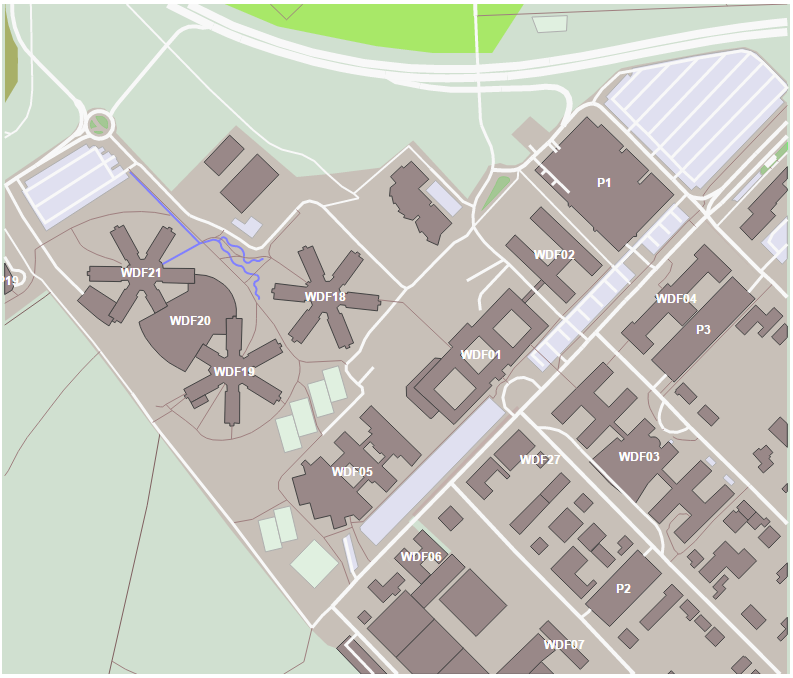
We also add in streams (-where "waterway IS NOT NULL"), and get this result:

Let's selectively add some labels to the buildings:
svg.selectAll(".buildingname")
.data(buildings.features)
.enter().append("text")
.attr("class", "buildingname")
.attr("transform", function(d) {
return "translate(" + path.centroid(d) + ")"; })
.attr("dy", ".35em")
.text(function(d) {
var id = d.id;
if(id){
if(id.indexOf("SAP W")===0){
return id.substring(4);
}
if(id.indexOf("P")===0){
return id;
}
}
return;
});
Basically, I don't want all building labels, because there are a lot of them, and - as will become apparent later - I only want the ones really that start with "SAP W". Since I don't really need the "SAP" bit either, we're only going to display what comes after (i.e. WDF01, WDF02, etc.). I also want the labels for the parking structures, to avoid confusion with other buildings, and helps with overall orientation of where what is. The positioning of the label is simply the center of the path that draws the building.
Adding data to visualize
While it is nice to be able to reproduce a map based on OSM data, it would be a lot more valuable to use this as a basis for adding additional visualization. We have a handle on each element in this map, and could for instance color the building any color we wish, or add a bubble on each building where size communicates some metric, for instance. What I decided to do was to look at the different Functional Areas of the SAP employees working in these buildings. So, I created a little CSV/Excel file with this data, and pulled it into my visualization by modifying my code to use require.js. This is also used by SAP Lumira to pull in additional resources, as I described in this article, so it can easily be turned it into a Lumira extension.
I decided to add a little column chart to each WDF building. The code for this is pretty simple, and is basically something like this but with an ordinal color scale to give each functional area a different color. I also suppress the x-axis labels, to keep things simple and clean, as the chart will be so small that the text will overlap anyway.
Probably the trickiest thing here was the positioning of the chart itself, and the easiest way is to simple create "g" tags based on the centroid (just like we did the labels).
var buildingchart_width = 75;
var buildingchart_height = 50;
svg.selectAll(".buildingchart")
.data(buildings.features)
.enter().append("g")
.attr("class", "buildingchart")
.attr("transform", function(d) {
return "translate(" + (path.centroid(d)[0] - (buildingchart_width/2)+10) + "," + (path.centroid(d)[1] - (buildingchart_height + 20)) + ")"; })
.attr("id", function(d) {
var id = d.id;
if(id){
if(id.indexOf("SAP W")===0){
return id.substring(4);
}
}
return;
});
Basically, this creates a "g" for every building, but only those where the name/id starts with "SAP W" do we actually add an "id" attribute. This way we can select any "g" attached to a relevant building using g#WDF01, etc.. The real trick is in the "translate" where we use the centroid (a point with x and y coordinates), add some offsets, so we basically have a 75x50 canvas for each WDF building in the map, centered a little above the building label. By then looping through the data and filtering by building, we create the same barchart for each building, but obviously with different data, appended to the correct "g" tag. Since there is a bit of imbalance in the employees per building, I am adjusting the y scale domain for each chart.

All we miss now is a legend so we know what each of the colored bars actually stand for, and this is basically just a little rectangle of the right color, followed by the name of the Functional Area. Add a title and we end up with our final result:
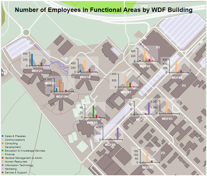
And again: all of this is SVG and CSS styling. If we don't like the color of something we can change it easily. If we want a different kind of chart for each building, no problem, we just replace the code that adds the column chart to the "g"s with something else.
I hope this gave a good overview of what is involved in building map-based visualizations from scratch based on OpenStreetMap.org maps, especially on low-scale or street level maps. We could have just had a series of bar charts with a text label, but that wouldn't convey how these buildings relate to each other.Placing this on a map makes it immediately more appealing, while adding additional information. Hopefully, seeing how this is done will encourage you to develop your own.
- SAP Managed Tags:
- SAP BusinessObjects Design Studio,
- SAP Lumira
1 Comment
You must be a registered user to add a comment. If you've already registered, sign in. Otherwise, register and sign in.
Labels in this area
-
ABAP CDS Views - CDC (Change Data Capture)
2 -
AI
1 -
Analyze Workload Data
1 -
BTP
1 -
Business and IT Integration
2 -
Business application stu
1 -
Business Technology Platform
1 -
Business Trends
1,661 -
Business Trends
86 -
CAP
1 -
cf
1 -
Cloud Foundry
1 -
Confluent
1 -
Customer COE Basics and Fundamentals
1 -
Customer COE Latest and Greatest
3 -
Customer Data Browser app
1 -
Data Analysis Tool
1 -
data migration
1 -
data transfer
1 -
Datasphere
2 -
Event Information
1,400 -
Event Information
64 -
Expert
1 -
Expert Insights
178 -
Expert Insights
270 -
General
1 -
Google cloud
1 -
Google Next'24
1 -
Kafka
1 -
Life at SAP
784 -
Life at SAP
11 -
Migrate your Data App
1 -
MTA
1 -
Network Performance Analysis
1 -
NodeJS
1 -
PDF
1 -
POC
1 -
Product Updates
4,578 -
Product Updates
323 -
Replication Flow
1 -
RisewithSAP
1 -
SAP BTP
1 -
SAP BTP Cloud Foundry
1 -
SAP Cloud ALM
1 -
SAP Cloud Application Programming Model
1 -
SAP Datasphere
2 -
SAP S4HANA Cloud
1 -
SAP S4HANA Migration Cockpit
1 -
Technology Updates
6,886 -
Technology Updates
395 -
Workload Fluctuations
1
Related Content
- ModuleError: failed to load 'unit/unitTests.qunit.js' in Technology Q&A
- How can I use Langsmith with SAP AI Core by selecting LLMs through what SAP provides me? in Technology Q&A
- How to pass parameter to getEntitySet from SAPUI5? in Technology Q&A
- 404 error while calling SAP Build Work Zone Notification API in BAS in Technology Q&A
- Unlocking Full-Stack Potential using SAP build code - Part 1 in Technology Blogs by Members
Top kudoed authors
| User | Count |
|---|---|
| 11 | |
| 10 | |
| 10 | |
| 10 | |
| 8 | |
| 7 | |
| 7 | |
| 7 | |
| 7 | |
| 6 |