
- SAP Community
- Products and Technology
- Technology
- Technology Blogs by SAP
- DMO: background on table split mechanism
Technology Blogs by SAP
Learn how to extend and personalize SAP applications. Follow the SAP technology blog for insights into SAP BTP, ABAP, SAP Analytics Cloud, SAP HANA, and more.
Turn on suggestions
Auto-suggest helps you quickly narrow down your search results by suggesting possible matches as you type.
Showing results for
Product and Topic Expert
Options
- Subscribe to RSS Feed
- Mark as New
- Mark as Read
- Bookmark
- Subscribe
- Printer Friendly Page
- Report Inappropriate Content
06-11-2015
12:11 PM
This blog explains the technical background of table split as part of the database migration option (DMO).
As a prerequisite, you should have read the introductionary document about DMO: Database Migration Option (DMO) of SUM - Introduction and the technical background in DMO: technical background.
During the migration of application tables, the migration of big tables might dominate the overall runtime. That is why SAPup considers table splitting to reduce the downtime of the DMO procedure. Table splitting shall prevent the case that all tables but a few have been migrated, and that only a small portion of all R3load processes these remaining (big) tables processes. The other R3load processes would be idle (to be more precise: would not run), and the long tail processing of the big tables would increase the downtime unnecessarily. See figure 1 below for a schematic view.

SAPup uses the following approach to define the tail: if the overall usage of R3load pairs (for export and import) drops below 90 %, SAPup handles all tables that are processed afterwards as being part of the tail (see figure 2 below).

During the configuration of the DMO procedure, you will configure a number of R3load processes, which determines the number of R3loads that may run in parallel. This explanation will talk about R3load pairs that are either active of idle, which is rather a virtual view. If an R3load pair did execute one job, it will not wait in status idle, but end. SAPup may then start another R3load pair. Still for the discussion of table split, we consider a fixed number of (potential) R3load pairs, which are either active or idle. The following figure 3 illustrates this view.

Automatic table splitting
SAPup will automatically determine the table split conditions, and there is no need and no recommendation to influence the table splitting. Your task is to find the optimal number of R3load processes during a test run, and provide the table duration files for the next run. (SAPup will use the table duration files to calculate the table splitting based on the real migration duration instead of the table size; see DMO guide, section 2.2 “Performance Optimization: Table Migration Durations”).
You may still want to learn more on the split logic, so this blog introduces some background on table splitting. Note that SAPup will not use R3ta for the table split.
Table split considerations
Typically, you will expect table splitting to happen for big tables only, but as we will see, the attempt to optimize the usage of all available (configured) R3load processes may result in splitting other tables as well. Still, splitting a table into too many pieces may result in a bad export performance: lots of parallel fragmented table segments will decrease read performance, and increase the load on the database server. A table may be big, but as long as has been completely processed before the tail processing starts, there is no reason to split that table. That is why the tool will calculate a minimum of table splits to balance all requirements.
The logic comprises four steps: table size determination, table sequence shuffling, table split determination, and assignment to buckets. A detailed explanation of the steps will follow below. During the migration execution, SAPup will organize tables and table segments in buckets, which are a kind of work packages for the R3load pair to export and import. During the migration phase, each R3load pair will typically work on several buckets, one after the other.
Step 1: Sorting by table size
SAPup will determine the individual table sizes, and then sort all tables descending by size.
In case you provide the table duration file from a previous run in the download folder, SAPup will use the table migration duration instead of the table size.

Assuming we only had sixteen tables, figure 4 above shows the sorted table list. The table number shall indicate the respective initial positioning in the table list.
Step 2: Shuffle table sequence
Migrating the tables in sequence of their size is not optimal, so the table sequence is reordered (“shuffled”) to achieve a good mixture of bigger and smaller application tables. Figure 5 below tries to illustrate an example.
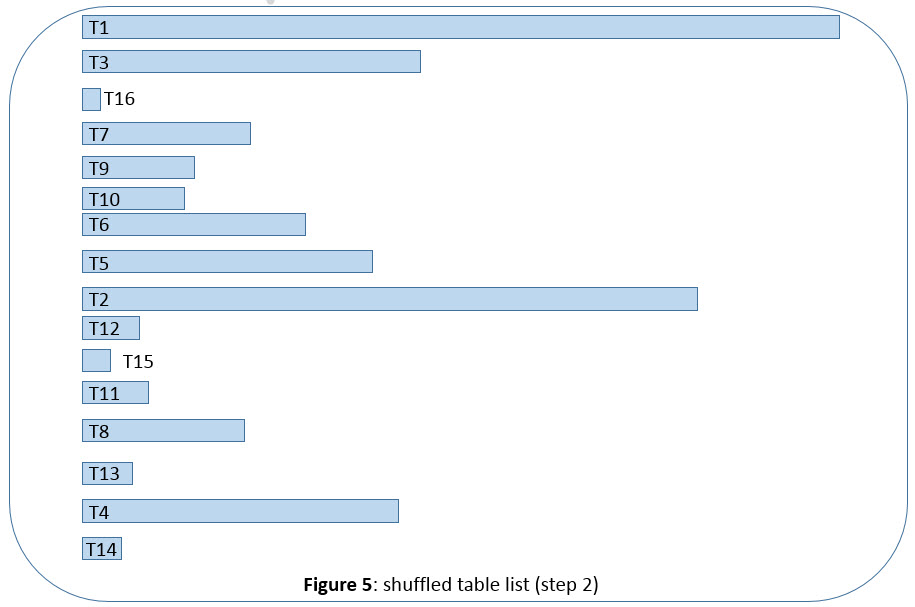
SAPup uses an internal algorithm to shuffle the table sequence, so that table sizes alternate between bigger and smaller.
Step 3: Table split determination
SAPup will now simulate table splitting, based on the number of configured R3load processes. Note that changing the number of configured R3load processes later during the migration phase will affect the runtime of the procedure.
For the simulation, SAPup will work on “slots” that represent the R3load pairs, and will distribute the tables from the shuffled table list into these slots. Note that these R3load “slots” are not identical to the buckets. SAPup will use buckets only at a later step. A slot is a kind of sum of all buckets, which are processed by an R3load pair.
Initially, the simulation will assign one table from the shuffled table list into each slot until all slots are filled with one table. In an example with only eight R3load pairs, this means that after the first eight tables, all slots have a table assigned, as shown in figure 6 below.
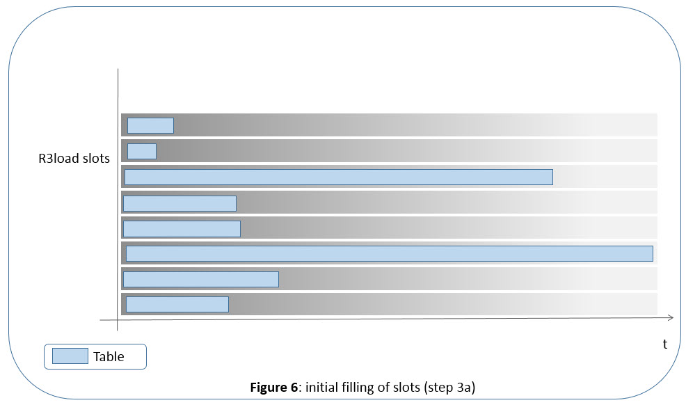
In our example, SAPup has filled all slots with one table, and the second slot from above has the smallest table, so it has the fewest degree of filling.
Now for all following assignments, SAPup will always assign the next table from the list to the slot that has the fewest degree of filling. In our example, SAPup would assign the next table (T7) to the second slot from top. After that, SAPup will most probably assign the next table (T9) to the first slot, see figure 7 below (sounds like Tetris, doesn’t it?).

Finally, SAPup has assigned all tables from the shuffled table list to the slots, as shown in figure 8 below. Note that the figures are not precise in reflecting the table sizes introduced in figure 4 and 5.

As last part of this simulation run, SAPup will now determine which tables to split. The goal is to avoid a long tail, so SAPup will determine the tail, and split all tables that are part of the tail.
SAPup determines the tail by the following calculation: SAPup sorts the slots by filling degree, and the tail begins at the point in time at which the usage of all R3load pairs is below 90%. All tables that are part of the tail – either completely or partially – are candidates for a split, as shown in figure 9 below. As an example, table T2 is shown as being part of the tail.

SAPup determines the number of segments into which the table will be split by the degree by which the table belongs to the tail. The portion of the table that does not belong to the tail is the scale for the table segments to be created. For the example of table T2, this may result in three segments T2/1, T2/2, and T2/3.
SAPup will now extend the shuffled table list by replacing the detected tables by its table segments. Figure 10 shows the example with three segments for table T2.

SAPup starts the next iteration of the simulation, based on the shuffled table list with table segments.
If the calculated tail is negligible (lower than a specific threshold) or if the third simulation has finished, SAPup will continue with step 4.
Step 4: Table and table segments assignment to buckets
The result of step 3 is a list of tables and table segments whose sequence does not correlated to the table size, and which was optimized to fill all R3load slots with a small tail. Now SAPup will work with buckets (work packages for R3load pairs) instead of slots. This is a slightly different approach, but as the filling of the buckets will use the same sequence of tables before, the assumption is that it has the same result.
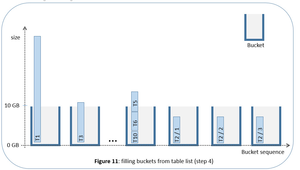
SAPup will assign the tables of this list to the buckets in the sequence of the list. The rules for this assignment are
- A bucket will get another table or table segment assigned from the list as long as the bucket size is lower than 10 GB.
- If the next table or table segment is bigger than 10 GB, the current bucket is closed, and SAPup will assign the table or table segment to next bucket.
- SAPup will put segments of a split table into different buckets– otherwise two table segments would reside in one bucket, which neutralizes the desired table split.
The first rule results in the effect that a bucket may have more table content than 10 GB. If a table of e.g. 30 GB was not determined for a split, the respective bucket will have this size.The second rule may result in the effect that a bucket is only filled to a low degree, if the following table / table segment was bigger than 10 GB so that it was put into the following bucket.The third rule results in the effect that e.g. for a table with four segments of size 5 GB each, several buckets will have a size of 5 GB. Figure 11 below tries to illustrate this with some examples.
Now SAPup has defined the distribution of tables and table segments into buckets, which in turn are part of a bucket list. All this happens during the phase EU_CLONE_MIG_DT_PRP for the application tables (and during phase EU_CLONE_MIG_UT_PRP for the repository). Note that the DT or UT part of the phase name is no indication whether or not the phase runs in uptime (UT) or downtime (DT): EU_CLONE_MIG_DT_PRP runs in uptime. The migration of application tables happens in downtime during phase EU_CLONE_MIG_DT_RUN. During the migration phase, SAPup will start the R3load pairs and assign the next bucket from the bucket list. As soon as an R3load pair is finished (and closes), SAPup will start another R3load pair and assign the next bucket to this pair, as shown in the following figure 12.

Relevant log files are
- EUMIGRATEDTPRP.LOG: tables to split, number of buckets, total size
- EUMIGRATEDTRUN.LOG: summary of migration rate
- MIGRATE_DT_RUN.LOG: details like R3load logs
Additional considerations
Typically, each R3load pair will execute more than one bucket. Exceptions may happen for small database sizes. As an example, for a total database size of 9992.3 MB and 20 R3load pairs (so 40 configured R3load processes), the tool would reduce the bucket size to put equal load to all R3load pairs. The log will contain a line such as “Decreasing bucket size from 10240 to 256 MB to make use of 160 processes”. Below you see the respective log entry in EUMIGRATEUTPRP.LOG:
1 ETQ399 Total size of tables/views is 9992.3 MB.
2 ETQ399 Decreasing bucket size from 10240 to 256 MB to make use of 20 processes.
…
1 ETQ000 ==================================================
1 ETQ399 Sorting 10801 tasks for descending sizes.
1 ETQ000 ==================================================
1 ETQ399 Distributing into 20 groups of size 500 MB and reshuffling tasks.
1 ETQ000 ==================================================
- SAP Managed Tags:
- Software Logistics - System Maintenance,
- Software Logistics
Labels:
30 Comments
You must be a registered user to add a comment. If you've already registered, sign in. Otherwise, register and sign in.
Labels in this area
-
ABAP CDS Views - CDC (Change Data Capture)
2 -
AI
1 -
Analyze Workload Data
1 -
BTP
1 -
Business and IT Integration
2 -
Business application stu
1 -
Business Technology Platform
1 -
Business Trends
1,658 -
Business Trends
93 -
CAP
1 -
cf
1 -
Cloud Foundry
1 -
Confluent
1 -
Customer COE Basics and Fundamentals
1 -
Customer COE Latest and Greatest
3 -
Customer Data Browser app
1 -
Data Analysis Tool
1 -
data migration
1 -
data transfer
1 -
Datasphere
2 -
Event Information
1,400 -
Event Information
66 -
Expert
1 -
Expert Insights
177 -
Expert Insights
299 -
General
1 -
Google cloud
1 -
Google Next'24
1 -
Kafka
1 -
Life at SAP
780 -
Life at SAP
13 -
Migrate your Data App
1 -
MTA
1 -
Network Performance Analysis
1 -
NodeJS
1 -
PDF
1 -
POC
1 -
Product Updates
4,577 -
Product Updates
344 -
Replication Flow
1 -
RisewithSAP
1 -
SAP BTP
1 -
SAP BTP Cloud Foundry
1 -
SAP Cloud ALM
1 -
SAP Cloud Application Programming Model
1 -
SAP Datasphere
2 -
SAP S4HANA Cloud
1 -
SAP S4HANA Migration Cockpit
1 -
Technology Updates
6,873 -
Technology Updates
422 -
Workload Fluctuations
1
Related Content
- Receive a notification when your storage quota of SAP Cloud Transport Management passes 85% in Technology Blogs by SAP
- CAP LLM Plugin – Empowering Developers for rapid Gen AI-CAP App Development in Technology Blogs by SAP
- Demystifying Transformers and Embeddings: Some GenAI Concepts in Technology Blogs by SAP
- Sharing SAP HANA Cloud instance to multiple subaccounts and creating HDI containers in Technology Blogs by Members
- Db2 Database Recovery and Cloud Object Store in Technology Blogs by SAP
Top kudoed authors
| User | Count |
|---|---|
| 40 | |
| 25 | |
| 17 | |
| 13 | |
| 7 | |
| 7 | |
| 7 | |
| 6 | |
| 6 | |
| 6 |