IBP for Supply Optimizer: the mathematics behind

[carsten_schumm]

Introduction

To find the cost-optimal solution, the optimizer transforms the IBP for Supply model into a mathematical representation. This representation is called Mixed-Integer Linear Program (MILP, see also Linear programming - Wikipedia, the free encyclopedia). This MILP can be solved to a mathematical proven optimal solution. A basic understanding of these MILPs is required for the further explanations.

Continuous variables

The variables in the model resemble the decisions, material flows and inventory-situation in the Supply plan:

• Production: each possible production gets its own variable, which equals the produced amount of the main output-product. For each period and production (P-rule) combination one variable is required.


• Transport: each possible transport inside the network or to a customer requires an own variable. They equal the transported amount of a distinct product over a transport-lane. For each period and transport C- and T-rules) one variable is required.


• External receipt/procurement: for each period and external receipt (U-rule) one variable is used to define the amount of procured material.


• Demand: for each consensus demand a variable resembles the satisfied amount. A helper variable with the non-delivered amount (demand quantity minus the satisfied amount) is used to penalize the non-deliveries in the objective function.


• Inventory: for each period, product and location-combination one variable reflects the current inventory level.

Binary variables

Currently two features of the model require binary decisions:

1. Minimum lot-sizes on transport and production: the optimizer needs to decide to transport resp. produce 0 or at least the minimum lot-size amount. Therefore a binary variable is required for each period to represent this decision.


2. Fix costs: similar to the minimum lot-sizes a decision variable is required for the fix costs in each period.

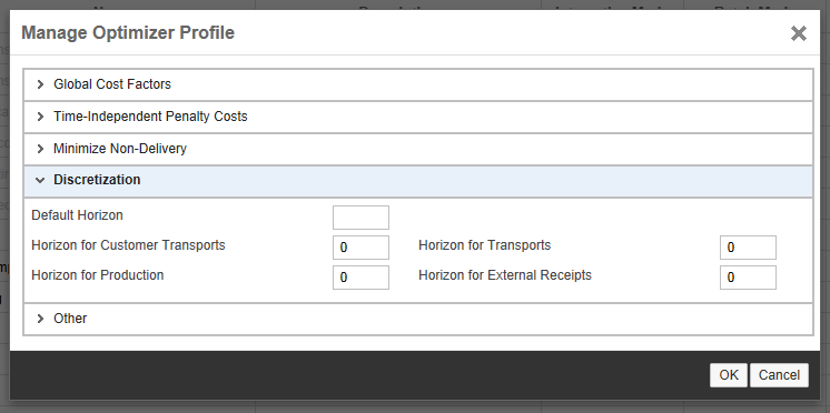
As binary (and integer) variables have a high impact on the MILP-solver runtime, it is recommended to avoid them as far as possible. By setting the discretization horizon in the optimizer profile it is possible to limit these binary decisions to the first periods in the planning horizon:

Constraints

The constraints in the mathematical model combine the variables with the business-logic of the Supply model:

• Stock-Balance equation: this equation ensures the integrity of the inventory level. It also ensures the correct material-flow and satisfaction of the bill-of-material for the Production-rules, as the same variables are used in the different equations. For each period, product and location combination it looks like this:
  inventory-level in period n =
      inventory-level in period n-1 // carry-over of previous period
      + incoming transports         // all transport arriving in this period
      + production receipts         // production-receipts (as main product or co-product)
      + external receipt            // procured amount
      - outgoing transports         // all transport leaving in this period
      - production component usage  // used amount for production of other products


• Resources: for all resources and periods a constraint ensures that the capacity of the resource is not exceeded:
  sum of resource-usages <= resource-capacity


• Adjusted and minimum values: These values set resp. restrict some of the decision variables. But as they can't be satisfied in all cases (e.g. due to missing material) they are modelled as semi-hard (often also called pseudo-hard) constraints. This avoids infeasibilities in the mathematical model. Due to very high costs for violations of these constraints they are usually all fulfilled.

Objective function

As our model is cost-based, the objective is of course to minimize these costs. Consequently the objective function contains all costs:

Objective function =

  all non-delivery variable costs

  + all transport variable costs

  + all transport fix costs

  + all production variable costs

  + all production fix costs

  + all external receipt variable costs

  + all external receipt fix costs

  + all inventory holding variable costs

  + all inventory target violation variable costs

  + all maximum inventory violation variable costs

Variable costs are based on the corresponding amount of the product. Sometimes they are also called rate costs.

Example: variable costs for transport of product P1 from location L1 to location L2 are 0.001 in period 3. If an amount of 100 is transported in this period, this results in 100 * 0.001 additional costs in the objective function.

Fix costs arise if an amount is greater than 0, but are independent of the amount itself.

Example: fix costs for transport of product P1 from location L1 to location L2 are 1.5 in period 2. If any amount greater than 0 is transported in this period, this results in additional costs of 1.5 in the objective function.

Note: The different cost-types can be multiplied with global cost-factors set in the optimizer profile:

Example: by setting the global cost-factor for External Receipt Variable Cost to a small value (e.g. 0.001), it is possible to check if the procurement costs hinder demand-satisfaction.

In the message-protocol the different parts of the objective function in the solution can be seen:

Additionally the objective function value and its bound are displayed. In some cases (e.g. decomposition used) the bound is not available.

Conclusion

This rough description hopefully eases the usage of the optimizer in IBP for Supply. Please let me know if further questions on this topic arise. Also please note that further blogs concerning the optimizer are planned during the next months.