
- SAP Community
- Products and Technology
- CRM and Customer Experience
- CRM and CX Blogs by Members
- Customer Activity Repository Intraday Forecast bas...
CRM and CX Blogs by Members
Find insights on SAP customer relationship management and customer experience products in blog posts from community members. Post your own perspective today!
Turn on suggestions
Auto-suggest helps you quickly narrow down your search results by suggesting possible matches as you type.
Showing results for
joshcu
Explorer
Options
- Subscribe to RSS Feed
- Mark as New
- Mark as Read
- Bookmark
- Subscribe
- Printer Friendly Page
- Report Inappropriate Content
05-23-2023
5:33 PM
Hi SAP fans!
This is my first SAP Blog and I hope my first entry would be a useful one. The information that I will share would hopefully supplement an existing blog about SAP CAR On Shelf Availability program /OSA/DISPATCHER already. This is the link of that topic https://blogs.sap.com/2019/12/17/sap-car-osa-on-shelf-availability/. However the context on how share the use of /OSA/DISPATCHER is on the use of it in tandem with CAR Unified Demand Forecast with respect to the standard HANA calculation view sap.is.ddf.udf.ifc IntradayForecast (in HDBSTUDIO). Why do we need this functionality this would help with better planning of articles with short shelf life (either freshly produced or externally sourced), and how this can help reduce food waste. This blog contains purely SAP Standard information, no custom development information nor logic was shared, and no affiliation to any company was shared as well.
I will try to explain the extent of the limitation and/or minimum requirements that the OSA program need to generate an intraweek pattern. When we generate forecast in general we need a historical pool of relevant data we need as basis of forecast. As the related blog post I have attached, indeed you need to be conscious if an article (material) is a fast selling article or slow selling article, since this will be the basis on how good the quality of each pattern per level would be in the end. Another factor to contribute to the quality of the pattern is granularity which I will talk about later. If the pattern that would be generated is at the level of:
If a certain article is not fast moving enough the program won’t be able to generate a level 1 pattern for it and would be then part of the historic data as basis of level 2.
For level 1, all historical POS data that pertains to the specific article and specific store, contributes to the quality of the pattern of the 1st level pattern. That pattern is also used by that specific article from that specific store. Now the minimum count of POS data needed to form this pattern, depends on what parameters in the profile you set in the /OSA/DISPATCHER program. Now comes the terminology Granularity. This number is taken into knowing what is the minimum POS transaction count an article is sold across a defined historical look-back period (Number of weeks, as show below). Note that we only count POS transaction that happened and not how many pieces were sold within each and every POS transaction. When doing your testing you can count the number of POS transactions in based on your look back period from table /DMF/TS_PS.
Note that there is a SAP standard note that can be applied to lower the granularity below 501, wherein you can now specifiy granularity from 21 to 5000. Just know what the implications are when you understand upon further reading of this blog. 3136126 - Extend the Granularity Range of the On-Shelf Availability Algorithm
The formula to know the minimum POS count for certain level is created is by
Granularity x (constant multiplier of 2.5 hard coded in the program)
604,800 / Granularity = seconds (you can convert to minutes) interval OSA pattern time slices
So example if my granularity is 336, it means 336*2.5 = 840; we need to reach this count of POS transaction per store-article within let us say we set 13 weeks look back period to be able create the most specific pattern. This minimum POS trnx count would also apply to the next level of pattern which is the store-merchandise category pattern. So if I theoretically say, within a group of articles belonging to 1 merchandise category, if lets say all of them are slow sellers and not a single article within that group sold 840 times within 13 weeks….. but collectively, when we count all POS transactions that occurred over a period of 13 weeks and they reached 840 or more, then the OSA program would create a merchandise category pattern. Hence the same logic goes for Store-Pattern level, but of course this pattern at this level is no longer desirable.
So if we analyze what would be a factor in deciding what granularity you would choose. You need to consider that it affects the required minimum POS transaction that an article needs to reach in order for the program to create a pattern. You can see here that you need more sales per day. So why do we increase granularity when it increases the minimum required POS count? Simple answer is that it gives us better quality pattern when we raise granularity.
Now going back to the context of my topic, this OSA pattern would be used in conjunction with UDF day (/DMF/UFC_TS) forecast to create an intraday forecast using the standard calculation view (sap.is.ddf.udf.ifc.IntradayForecast). However, I would like to highlight one limitation that the standard calculation view have as the time of this writing. That the merchandise group level pattern is not utilized, though there is a merchandise pattern generated. Therefore you need to customize a copy of this standard calculation view if you want to consider utilizing the merchandise category pattern.
I have included some screenshot of the standard calculation view of intradayforecast and how to try it out in an ad-hoc run with manual input parameters. You can of course imagine the application for this when utilized in your own CDS and expose it through OData service to a UI application.
sap.is.ddf.udf.ifc.IntradayForecast
Date range you enter here is in this format YYYYMMDD, note that the date range here is the forecast dates, hence enter future dates(example: tomorrow to tomorrow+7). Note that the OSA pattern creates a 7 days pattern.
Slot Time Frame (in terms of minutes) is per how many time slices breakdown of the intraday forecast you want to generate.(example 60 means an hourly intraday forecast result)
Store ID, to limit search results.
Note that results will be shown, if we have entries in UDF forecast value (in terms of base unit of measure) in /DMF/UFC_TS. We have OSA pattern (7-day pattern) /osa/iw_pattern, the latest run id pattern would be used. In saying this for as long as you have an OSA pattern regardless if the run is from an old one (say you ran OSA program a month ago or longer), the calculation view will used the latest run id.
Hope this blog would give you a good level of insight on this subject matter!
This is my first SAP Blog and I hope my first entry would be a useful one. The information that I will share would hopefully supplement an existing blog about SAP CAR On Shelf Availability program /OSA/DISPATCHER already. This is the link of that topic https://blogs.sap.com/2019/12/17/sap-car-osa-on-shelf-availability/. However the context on how share the use of /OSA/DISPATCHER is on the use of it in tandem with CAR Unified Demand Forecast with respect to the standard HANA calculation view sap.is.ddf.udf.ifc IntradayForecast (in HDBSTUDIO). Why do we need this functionality this would help with better planning of articles with short shelf life (either freshly produced or externally sourced), and how this can help reduce food waste. This blog contains purely SAP Standard information, no custom development information nor logic was shared, and no affiliation to any company was shared as well.
- Batch job Program: /OSA/DISPATCHER
- Transaction code: /OSA/DISPATCH
- Tables:
- /osa/iwp_conf – contains the run id, store number, date/time of the run, historical scope date range and what configuration/profile was used during that run.
- /osa/iw_pattern - Pattern details, run id, article, subdepartment id (merchandise category, product id.
- /DMF/UFC_TS – UDF day forecast value per product – location combination.
- /DMF/PROD_EXT_XR – to get the product GUID given the SAP Material number
- /DMF/LOC_EXT_XR – to get the location GUID given the store number
- Profile configuration: Long path > SAP Customer Activity Repository > On-Shelf Availability > Initialize On-Shelf Availability Algorithm (Configuration)
I will try to explain the extent of the limitation and/or minimum requirements that the OSA program need to generate an intraweek pattern. When we generate forecast in general we need a historical pool of relevant data we need as basis of forecast. As the related blog post I have attached, indeed you need to be conscious if an article (material) is a fast selling article or slow selling article, since this will be the basis on how good the quality of each pattern per level would be in the end. Another factor to contribute to the quality of the pattern is granularity which I will talk about later. If the pattern that would be generated is at the level of:
- store-article
- store-merchandise category
- store level
If a certain article is not fast moving enough the program won’t be able to generate a level 1 pattern for it and would be then part of the historic data as basis of level 2.
For level 1, all historical POS data that pertains to the specific article and specific store, contributes to the quality of the pattern of the 1st level pattern. That pattern is also used by that specific article from that specific store. Now the minimum count of POS data needed to form this pattern, depends on what parameters in the profile you set in the /OSA/DISPATCHER program. Now comes the terminology Granularity. This number is taken into knowing what is the minimum POS transaction count an article is sold across a defined historical look-back period (Number of weeks, as show below). Note that we only count POS transaction that happened and not how many pieces were sold within each and every POS transaction. When doing your testing you can count the number of POS transactions in based on your look back period from table /DMF/TS_PS.
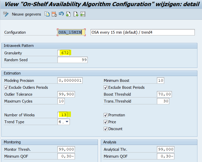
OSA Algorithm configuration 15 minutes

OSA Algorithm Configuration 20 minutes

OSA Algorithm Configuration 30 minutes
Note that there is a SAP standard note that can be applied to lower the granularity below 501, wherein you can now specifiy granularity from 21 to 5000. Just know what the implications are when you understand upon further reading of this blog. 3136126 - Extend the Granularity Range of the On-Shelf Availability Algorithm
The formula to know the minimum POS count for certain level is created is by
Granularity x (constant multiplier of 2.5 hard coded in the program)
604,800 / Granularity = seconds (you can convert to minutes) interval OSA pattern time slices
So example if my granularity is 336, it means 336*2.5 = 840; we need to reach this count of POS transaction per store-article within let us say we set 13 weeks look back period to be able create the most specific pattern. This minimum POS trnx count would also apply to the next level of pattern which is the store-merchandise category pattern. So if I theoretically say, within a group of articles belonging to 1 merchandise category, if lets say all of them are slow sellers and not a single article within that group sold 840 times within 13 weeks….. but collectively, when we count all POS transactions that occurred over a period of 13 weeks and they reached 840 or more, then the OSA program would create a merchandise category pattern. Hence the same logic goes for Store-Pattern level, but of course this pattern at this level is no longer desirable.
So if we analyze what would be a factor in deciding what granularity you would choose. You need to consider that it affects the required minimum POS transaction that an article needs to reach in order for the program to create a pattern. You can see here that you need more sales per day. So why do we increase granularity when it increases the minimum required POS count? Simple answer is that it gives us better quality pattern when we raise granularity.
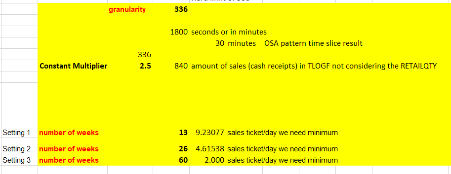
Computation for granularity 336 or 30 minutes sampling

Computation for granularity 672 or 15 minutes sampling (more granular, better accuracy, better pattern, however higher historical POS sales transaction required)
Now going back to the context of my topic, this OSA pattern would be used in conjunction with UDF day (/DMF/UFC_TS) forecast to create an intraday forecast using the standard calculation view (sap.is.ddf.udf.ifc.IntradayForecast). However, I would like to highlight one limitation that the standard calculation view have as the time of this writing. That the merchandise group level pattern is not utilized, though there is a merchandise pattern generated. Therefore you need to customize a copy of this standard calculation view if you want to consider utilizing the merchandise category pattern.
I have included some screenshot of the standard calculation view of intradayforecast and how to try it out in an ad-hoc run with manual input parameters. You can of course imagine the application for this when utilized in your own CDS and expose it through OData service to a UI application.
sap.is.ddf.udf.ifc.IntradayForecast

Standard intradayForecast HANA DB calculation view

Ad-hoc run entering manually variable inputs to see intraday forecast results
Date range you enter here is in this format YYYYMMDD, note that the date range here is the forecast dates, hence enter future dates(example: tomorrow to tomorrow+7). Note that the OSA pattern creates a 7 days pattern.
Slot Time Frame (in terms of minutes) is per how many time slices breakdown of the intraday forecast you want to generate.(example 60 means an hourly intraday forecast result)
Store ID, to limit search results.
Note that results will be shown, if we have entries in UDF forecast value (in terms of base unit of measure) in /DMF/UFC_TS. We have OSA pattern (7-day pattern) /osa/iw_pattern, the latest run id pattern would be used. In saying this for as long as you have an OSA pattern regardless if the run is from an old one (say you ran OSA program a month ago or longer), the calculation view will used the latest run id.
Hope this blog would give you a good level of insight on this subject matter!
- SAP Managed Tags:
- SAP Customer Activity Repository
You must be a registered user to add a comment. If you've already registered, sign in. Otherwise, register and sign in.
Labels in this area
-
ABAP
1 -
API Rules
1 -
c4c
1 -
CAP development
1 -
clean-core
1 -
CRM
1 -
Custom Key Metrics
1 -
Customer Data
1 -
Determination
1 -
Determinations
1 -
Introduction
1 -
KYMA
1 -
Kyma Functions
1 -
open SAP
1 -
RAP development
1 -
Sales and Service Cloud Version 2
1 -
Sales Cloud
1 -
Sales Cloud v2
1 -
SAP
1 -
SAP Community
1 -
SAP CPQ
1 -
SAP CRM Web UI
1 -
SAP Customer Data Cloud
1 -
SAP Customer Experience
1 -
SAP CX
1 -
SAP CX extensions
1 -
SAP Integration Suite
1 -
SAP Sales Cloud v2
1 -
SAP Service Cloud v2
1 -
SAP Service Cloud Version 2
1 -
Service and Social ticket configuration
1 -
Service Cloud v2
1 -
side-by-side extensions
1 -
Ticket configuration in SAP C4C
1 -
Validation
1 -
Validations
1
Related Content
- Creating your Local PPS Box with SAP CARAB in CRM and CX Blogs by SAP
- AI capabilities in SAP CX in CRM and CX Blogs by Members
- Unleashing Customer Insights: SAP CDP for Retail in CRM and CX Blogs by SAP
- Partner Event Success: Celebrating the Launch of SAP Sales and Service Cloud v2 in CRM and CX Blogs by SAP
Top kudoed authors
| User | Count |
|---|---|
| 1 | |
| 1 | |
| 1 | |
| 1 | |
| 1 |