
- SAP Community
- Products and Technology
- Technology
- Technology Blogs by SAP
- ST05: Aggregate Trace Records
Technology Blogs by SAP
Learn how to extend and personalize SAP applications. Follow the SAP technology blog for insights into SAP BTP, ABAP, SAP Analytics Cloud, SAP HANA, and more.
Turn on suggestions
Auto-suggest helps you quickly narrow down your search results by suggesting possible matches as you type.
Showing results for
Advisor
Options
- Subscribe to RSS Feed
- Mark as New
- Mark as Read
- Bookmark
- Subscribe
- Printer Friendly Page
- Report Inappropriate Content
05-17-2023
10:23 AM
This is a follow-up to my blog post ST05: Basic Use. Here I explain various options for aggregating trace records. They greatly facilitate the analysis of a trace.
If you have not yet done so, please read the introductory post Use ST05 to Monitor the Communication of the ABAP Work Process with External Resources. There I describe how my measurement transactions
Fig. 1 shows the ALV list of Trace Main Records for the Audit Journal Fiori application F0997, with records for the interface types SQL, Enqueue, HTTP, and RFC. Refer to my blog post ST05: Basic Use for a complete description of the scope and purpose of the Trace Main Records. With its chronological sort order, the list provides a comprehensive picture of the flow of the application's communication with external agents, but it does not draw your attention to the most expensive statements, nor does it indicate events that have been executed multiple times or even redundantly. It also does not distinguish between statements related to the involved technical frameworks and statements that contribute to the business logic.
The main benefit of trace aggregation is for trace types SQL and BUF. They record concrete values used in individual statements, leading to a large variety of trace records. Aggregation creates a significantly shorter list of records, giving you a much better overview of the various kinds of statements and their durations or resource consumptions.
The list of Structure-Identical Statements (Fig. 2) summarizes identical Trace Main Records without considering the actual values for any bind variables. The resulting list is augmented by some statistics on the set of main records contributing to each entry, and (for SQL, BUF, and ENQ trace records) by metadata from the ABAP dictionary on the affected table, view, or lock object. Table 2 covers the columns that are shown in the default ALV grid layout. You may add a few additional fields with more technical content (e.g., from the SAP extended passport) by changing the list's layout.
The sort order is descending by Duration, placing the most expensive statements at the top. They have the biggest impact on the application's end-to-end response time and are your first entry point to a detailed analysis, which shall also consider the number of Records affected by the statement:
If Min. Duration / Record exceeds 10,000 µs = 10 ms for
Other purely technical indicators for potential improvements related to SQL trace records are
With domain knowledge about the application's business logic and its purpose, you may identify further critical statements by looking at
With button Absolute <-> Relative Values you can toggle between these two options for columns Executions, Duration, CPU Time, and Records. The relative values are expressed as percentages of the respective totals.
The drop-down menu of button Break Down Trace Record allows you to view either the contributing Trace Main Records or the associated Value-Identical Statements for selected list entries.
The list of Value-Identical Statements is sorted descending by Duration. Records with Execution = 1 are suppressed.
Value-identical SQL statements read the same data multiple times from the database, thus create unnecessary load. Identical data can be read redundantly by statements that are not value-identical―and not even structure-identical. This is not visible in the list of Value-Identical Statements. All unnecessary accesses to the persistence layer must be eliminated. This is a more comprehensive demand than just removing value-identical SQL statements. Unfortunately, there is no support in
Click button Break Down Trace Record to see the Trace Main Records contributing to the selected Value-Identical Statements.
The Table Accesses aggregation (Fig. 4) combines statements by their type, separately for each object. It aggregates all SQL trace records corresponding to statements of the same category (e.g.,
The list is sorted ascending by Object Name, category of Statement, and Connection Name.
The Table Accesses display provides a highly condensed survey of the tables with which the traced application works and how the application affects these tables. Use it to verify that there are no expensive accesses to tables that have no relevance to the business process, and to make sure that the required accesses have good performance.
As in the list of Structure-Identical Statements, button Absolute <-> Relative Values toggles between these options for columns Duration, CPU Time, Records, and Executions.
Use this enriched list of Table Accesses to understand the software domains used—either directly or via intermediary frameworks—by your application, and to assess how much they impact your application's performance. It may also uncover unnecessary accesses, which you can eliminate without breaking your application's functional correctness.
The Trace Overview (Fig. 6) provides a quality control of the trace, and also a high-level analysis to indicate potential problem areas. Use this aggregation option to convince yourself that the trace is reliable and to obtain a quick survey of the variety of recorded statements. This may give you some guidance for more detailed analyses.
It is divided into several areas:
The Sizing Information (Fig. 7) covers only changing database accesses, specifically
Your storage system sizing must be based on a trace that covers the entire business process with all user interaction steps from end to end. Do not apply any filter conditions while recording the trace.
The top of the Sizing Information contains the main characteristics of the system, identical to the top row in the Trace Overview (Fig. 6).
Section Number of
The next area, Size of Tables, Primary Keys, and Secondary Indexes, summarizes the static sizes in Bytes of the changed tables, including their indexes. It also indicates whether tables or indexes contain fields of type
Based on this information, section Estimation of Data Volume Added approximates the change to the database's overall size by the statements recorded in the trace: For each table its length plus the lengths of its indexes are summed up. These table-specific sums are then multiplied by either number of changed rows (as explained above) and the resulting sets of products are totalled and given in Bytes, kBytes, and MBytes. Typically, these values are lower limits for the change in the stored data volume, but in some situations may be overestimates. To guard against negative consequences of storage system under-sizing, you should always consider them lower limits, and try to assess the additional impact of the table fields whose sizes are not statically known. From previous experience, you may know their average size in typical production systems.
The Trace Single Records are sorted chronologically. The main value of this full resolution view on the trace records is mostly as an entry point to a technical analysis of how the database server or the buffers on the application server instances have handled table accesses via (Open) SQL statements. Investigations from a business logic perspective hardly ever work with the Trace Single Records.
Compared to the default list of chronologically sorted Trace Main Records, the various aggregation levels offered by
The high-level Trace Overview provides a very basic quality control of the trace recording. It can also identify performance bugs of the application, and it signals suspicious database accesses.
The Table Accesses view indicates with which tables your application works and what categories of statements it uses on these tables. Use it with your knowledge of the underlying business logic to detect unnecessary or expensive table accesses.
The list of Structure-Identical Statements focusses on statements with a common form and indicates slow statements or statements that are better handled by the application server instances' buffers. The list of Value-Identical Statements concentrates even stronger on redundant, therefore superfluous, statements with the same bind variable values. You must eliminate them to accelerate your application and to take load away from the central database server.
The Sizing Information has a different objective and supports the forecast of the required storage capacity by estimating how much the changing SQL statements of an application change the persisted data volume.
If you have not yet done so, please read the introductory post Use ST05 to Monitor the Communication of the ABAP Work Process with External Resources. There I describe how my measurement transactions
STATS and STATS_FE help you to detect performance bugs in your applications, and I state that ST05 is an essential analysis tool to find root causes for applications that are too slow or consume too many resources. In particular, ST05 captures requests and data transmissions between the ABAP work process and external components. By default these transmissions are not recorded to not incur the associated overhead. You need to consciously and explicitly activate the recording, and subsequently must switch it off. Once you have a high quality trace of your application's communication with external resources, you want to evaluate it in the most efficient way.Fig. 1 shows the ALV list of Trace Main Records for the Audit Journal Fiori application F0997, with records for the interface types SQL, Enqueue, HTTP, and RFC. Refer to my blog post ST05: Basic Use for a complete description of the scope and purpose of the Trace Main Records. With its chronological sort order, the list provides a comprehensive picture of the flow of the application's communication with external agents, but it does not draw your attention to the most expensive statements, nor does it indicate events that have been executed multiple times or even redundantly. It also does not distinguish between statements related to the involved technical frameworks and statements that contribute to the business logic.
Figure 1: In the chronologically sorted list of Trace Main Records, each entry corresponds to one execution of an ABAP statement calling an external resource, or to the processing of an incoming request.
To remedy these shortcomings,ST05 offers various options to summarize the list of Trace Main Records, which make your work with previously recorded traces much more efficient. They are all accessible from the drop-down menu of button Aggregate Trace ![]() . Table 1 briefly introduces them, and the following sections describe them in detail.
. Table 1 briefly introduces them, and the following sections describe them in detail.
| Structure-Identical Statements | Specific values of bind variables are not considered. |
| Value-Identical Statements | Structure-identical statements where the bind variables have the same values. |
| Table Accesses | Database accesses from the same category (SELECT, INSERT, UPDATE, DELETE, ...) grouped by object and by database connection.Buffer accesses using the same number of key fields. (Only for trace types SQL, BUF.) |
| Trace Overview | Quality control of the trace, break-down of records by type, and high-level evaluation with hints for potential optimizations. |
| Sizing Information | Estimates the data volume added by the traced application to the database. |
| Trace Single Records | Resolves individual low-level operations. (They are recorded only for trace types SQL, BUF.) |
The main benefit of trace aggregation is for trace types SQL and BUF. They record concrete values used in individual statements, leading to a large variety of trace records. Aggregation creates a significantly shorter list of records, giving you a much better overview of the various kinds of statements and their durations or resource consumptions.
Structure-Identical Statements
The list of Structure-Identical Statements (Fig. 2) summarizes identical Trace Main Records without considering the actual values for any bind variables. The resulting list is augmented by some statistics on the set of main records contributing to each entry, and (for SQL, BUF, and ENQ trace records) by metadata from the ABAP dictionary on the affected table, view, or lock object. Table 2 covers the columns that are shown in the default ALV grid layout. You may add a few additional fields with more technical content (e.g., from the SAP extended passport) by changing the list's layout.
Figure 2: The list of Structure-Identical Statements summarizes the Trace Main Records for statements with the same structure, but potentially distinct values for bind variables. The list is sorted descending by Duration.
| Executions | Total number of executions of the structure-identical statements. |
| Redundancy | Absolute number of redundant value-identical statements. |
| Identical | Relative number of redundant value-identical statements. |
| Duration | Total elapsed execution time in µs of the structure-identical statements. (Measured by the ABAP work process.) |
| CPU Time | Total HANA CPU time in µs used during the structure-identical statements' executions. (Only for SQL trace records on SAP HANA.) (Measured by the SAP HANA DB server.) |
| Memory | Maximum memory consumption in kByte during the structure-identical statements' executions. (Only for SQL trace records on SAP HANA.) (Measured by the SAP HANA DB server.) |
| Records | Total number of records affected by the structure-identical statements. (SQL, BUF: number of table or view rows; ENQ: number of lock granules) (Not for RFC, HTTP, APC, and AMC trace records.) |
| Duration / Execution | Average execution time in µs per contributing statement. |
| Records / Execution | Average number of records affected per contributing statement. |
| Duration / Record | Average execution time in µs per record. (Records = 0 ⇒ average execution time per contributing statement.) |
| Min. Duration / Record | Minimum execution time in µs per record. (Records = 0 ⇒ minimum execution time of contributing statements.) |
| Length | ABAP dictionary record length in Byte of the table or view. (Only for SQL and BUF trace records.) |
| Buffer Type | Buffer type of the table or view. (Only for SQL and BUF trace records.) |
| Table Type | Table type of the table or view. (Only for SQL and BUF trace records.) |
| Data Class | Type of data stored in the table. (Only for SQL and BUF trace records.) |
| Size | Estimated size category of the table. (Only for SQL and BUF trace records.) |
| Object Name | Name of the object that was accessed. (SQL, BUF: table or view; ENQ: lock object; RFC: function; HTTP, APC: path; AMC: channel ID) |
| Statement | Edited statement. (SQL: field list and FROM clause removed, variable names as place holders for values;BUF: buffer type, length of key values in characters, buffer operation; ENQ: lock operation, lock mode, table, granule argument; RFC: source, destination, CLIENT or SERVER, function, sent data in Byte;HTTP: method, status code, status text, scheme, host, port, CLIENT or SERVER, path;APC: executed action, protocol, host, port, CLIENT or SERVER, path;AMC: <empty>) |
The sort order is descending by Duration, placing the most expensive statements at the top. They have the biggest impact on the application's end-to-end response time and are your first entry point to a detailed analysis, which shall also consider the number of Records affected by the statement:
If Min. Duration / Record exceeds 10,000 µs = 10 ms for
SELECTs, or 50,000 µs = 50 ms for INSERTs, UPDATEs, or DELETEs, the statement's execution on the database is slow and shall be investigated in detail. If a statement has been executed multiple times (e.g., Executions ≥ 10), also consider the value of average Duration / Record. With few executions, a single outlier may distort the average, i.e., one slow execution may conceal several fast executions, but with 10 or more executions, it should be reliable and taken seriously. In my blog post Analyze Individual Trace Records, I explain how you can recognize the database's processing of a slow statement and how this may indicate optimization approaches.Other purely technical indicators for potential improvements related to SQL trace records are
- Column Buffer Type
It shall be empty. If a table's technical settings is Buffering switched on, the vast majority of Open SQL statements against this table shall be handled by the table buffer on the application server instance. Then they will not be recorded by an SQL trace. SQL trace records where Buffer Type equalsFUL,GEN, orSNGindicate that the table buffer was bypassed, which slows down the application, puts unnecessary load on the database server, and does not take advantage of the application server memory used to buffer the table's rows. Rewrite the corresponding statements so that they can be handled by the table buffer. Values in the Buffer Type column starting withDErepresent the technical setting Buffering allowed but switched off. Check whether buffering can be switched on for the affected tables. The Buffer TypeCUSTidentifies accesses to unbuffered customizing tables (Data Class =APPL2). Consider to switch on buffering for the table—this is typically suitable for customizing data. Finally, the entryDDICin the Buffer Type column indicates direct accesses to tables belonging to the ABAP dictionary. Replace them by using functionsDDIF*, in particularDDIF_NAMETAB_GETorDDIF_FIELDINFO_GET. - Columns Redundancy or Identical
They shall contain only zeros. These columns show the absolute number or relative number, respectively, of redundant Value-Identical Statements within the corresponding set of Structure-Identical Statements. These duplicate Value-Identical Statements repeatedly access the same rows on the database, instead of taking their content from the application's state in the application server instance. This is slower than necessary and wastes precious resources on the database server. You need to eliminate them. Refer to the following section on Value-Identical Statements for a complete discussion. - Columns Executions and Records / Execution
Entries with a large number of Executions and Records / Execution ≈ 1 may indicate single row SQL statements nested inside a loop. Consider a mass-enabled approach to reduce the number of data transfers.
With domain knowledge about the application's business logic and its purpose, you may identify further critical statements by looking at
- Columns Object Name and Statement
For SQL trace records: Does the application need rows from the table or view? If yes, is the statement'sWHEREclause as restrictive as possible, and does the field list request only necessary columns?
For the other trace types, similar questions apply and help to identify potentially unnecessary communication events triggered by your application. - Column Executions
Are all executions required for the application to be functionally correct? - Column Records
Does the number of rows make sense? Are all the records needed by the application? Can you use code push-down (at least in the form of SQL aggregate functions) to calculate on the database instead of transferring many rows to the ABAP work process?
With button Absolute <-> Relative Values
The drop-down menu of button Break Down Trace Record
Value-Identical Statements
The list of Value-Identical Statements (Fig. 3) also summarizes identical Trace Main Records, but unlike the Structure-Identical Statements, it takes the concrete values for any bind variables into account. This aggregation supports only SQL, BUF, and ENQ trace records. These are the only trace types where values are recorded. The columns in the list of Value-Identical Statements are mostly like the ones for the Structure-Identical Statements. Table 3 contains the differences.
Figure 3: The list of Value-Identical Statements summarizes Trace Main Records for statements with the same structure, and with identical values for bind variables. The list is sorted descending by Duration.
| Executions | Total number of executions of the value-identical statements. |
| Redundancy | Not available—covered by Executions. |
| Identical | Not available—covered by Executions. |
| Statement | Edited statement. (SQL: field list and FROM clause removed, variable values;BUF: buffer type, length of key values in characters, key values; ENQ: lock operation, lock mode, table, granule argument) |
The list of Value-Identical Statements is sorted descending by Duration. Records with Execution = 1 are suppressed.
Value-identical SQL statements read the same data multiple times from the database, thus create unnecessary load. Identical data can be read redundantly by statements that are not value-identical―and not even structure-identical. This is not visible in the list of Value-Identical Statements. All unnecessary accesses to the persistence layer must be eliminated. This is a more comprehensive demand than just removing value-identical SQL statements. Unfortunately, there is no support in
ST05 (nor in any other tool) to find all superfluous SQL statements.Click button Break Down Trace Record
Table Accesses
The Table Accesses aggregation (Fig. 4) combines statements by their type, separately for each object. It aggregates all SQL trace records corresponding to statements of the same category (e.g.,
SELECT, INSERT, UPDATE, DELETE) that access a table or view over the same logical database connection. Similarly, all BUF trace records triggered by statements that were handled by the table buffer or by other buffers on the application server instance, and that access an object with the same number of key fields are aggregated. No other trace types are supported by this aggregation option. Table 4 contains the fields displayed in the Table Accesses list.Figure 4: The list of Table Accesses summarizes, separately for each table or view, all statements of the same category. The sort order is alphabetically by Object Name, Statement category, and Connection Name.
| Object Name | Name of the table or view that was accessed. |
| Length | ABAP dictionary record length in Byte of the table or view. |
| Buffer Type | Buffer type of the table or view. |
| Table Type | Table type of the table or view. |
| Data Class | Type of data stored in the table. |
| Size | Estimated size category of the table. |
| Statement | Category of statement SQL: SELECT, INSERT, UPDATE, DELETE, ...BUF: buffer type, key length |
| Connection Name | Name of the logical database connection used by the contributing statements. |
| Duration | Total elapsed execution time in µs of the contributing statements. (Measured by the ABAP work process.) |
| CPU Time | Total HANA CPU time in µs used during the contributing statements' executions. (Only for SQL trace records on SAP HANA.) (Measured by the SAP HANA DB server.) |
| Memory | Maximum memory consumption in kByte during the contributing statements' executions. (Only for SQL trace records on SAP HANA.) (Measured by the SAP HANA DB server.) |
| Records | Total number of table or view rows affected by the contributing statements. |
| Executions | Total number of executions of contributing statements. |
The list is sorted ascending by Object Name, category of Statement, and Connection Name.
The Table Accesses display provides a highly condensed survey of the tables with which the traced application works and how the application affects these tables. Use it to verify that there are no expensive accesses to tables that have no relevance to the business process, and to make sure that the required accesses have good performance.
As in the list of Structure-Identical Statements, button Absolute <-> Relative Values
Button Component Hierarchy ![]() enhances the list of the Table Accesses (Fig. 5). It groups the accessed tables by their application component (levels 0 and 1 are supported, level 0 is the default, buttons
enhances the list of the Table Accesses (Fig. 5). It groups the accessed tables by their application component (levels 0 and 1 are supported, level 0 is the default, buttons ![]() or
or ![]() toggle between the levels), and additionally shows the tables’ short descriptions from the ABAP data dictionary. For each application component, absolute and relative subtotals of the duration, the number of records, and the number of executions are given separately for the statement categories (
toggle between the levels), and additionally shows the tables’ short descriptions from the ABAP data dictionary. For each application component, absolute and relative subtotals of the duration, the number of records, and the number of executions are given separately for the statement categories (SELECT, INSERT, UPDATE, DELETE; buffer accesses), and across all categories. 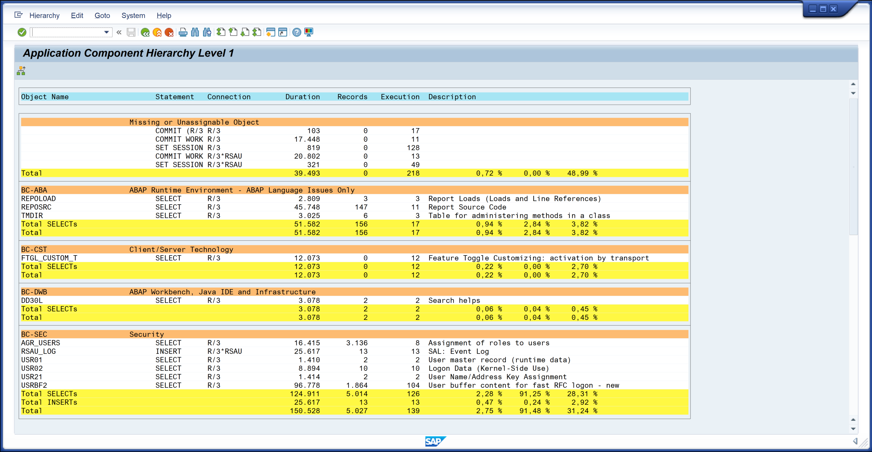
Figure 5: The Application Component Hierarchy view augments the list of Table Accesses (Fig. 4) by including the tables' application components and descriptions. With this additional information you can better understand why the tables are accessed when the application executes. The grouping by application component helps you to judge the run time contributions of the components.
Use this enriched list of Table Accesses to understand the software domains used—either directly or via intermediary frameworks—by your application, and to assess how much they impact your application's performance. It may also uncover unnecessary accesses, which you can eliminate without breaking your application's functional correctness.
Trace Overview
The Trace Overview (Fig. 6) provides a quality control of the trace, and also a high-level analysis to indicate potential problem areas. Use this aggregation option to convince yourself that the trace is reliable and to obtain a quick survey of the variety of recorded statements. This may give you some guidance for more detailed analyses.
Figure 6: The Trace Overview evaluates the trace's technical quality, and identifies performance bugs.
It is divided into several areas:
- At the top, the main characteristics of the system are shown. This corresponds to the situation when and where the Trace Overview was called. It is not necessarily related to the circumstances in which the application was executed and traced. This is particularly true for old traces from the trace directory, and even more so for traces imported from other systems.
Then, the time intervals between start and end of the trace analysis period and between the first and the last trace records are compared. A large discrepancy may indicate that the trace is incomplete. - The next part evaluates the trace’s technical quality and reliability. If it contains
ROLLBACKs,OPENoperations, or SQL statements that load content into the table buffer on the application server instance, you have not executed enough pre-runs of your application before recording the trace. The Trace Overview then advises you to Consider re-recording the trace. Before doing so, execute the application several times. Typically, you want to analyze and eventually optimize the repeated executions of your applications. For them, there should not be anyROLLBACKs. Also, all SQL statements should already be in the database server’s statement cache so that noOPENoperation is needed, and the table buffer should contain all necessary rows. - The following region condenses the trace by the records’ types (SQL, BUF, ENQ, ...), and within the types resolves the main statement categories. Values for Executions, Duration, and Records are given as absolute numbers and as percentages of the respective totals.
- Finally, the trace is analyzed for violations of common best practices to identify problematic or suspicious patterns like unnecessary accesses to the persistence layer, e.g.,
SELECTs for buffered tables or redundant DB accesses. Additionally, the SQL trace records are checked by Code Inspector to find statements whose access times to the persistence may erroneously depend on the amount of data persisted. This is typically a consequence of inadequate index support.
One section also deals with accesses to CDS views, to ensure that analytical CDS views are not used in transactional applications. If the trace contains SQL statements that access transactional CDS views, this section also suggest that you verify the modelling of these views. It must guarantee that SQL queries using them have response times and CPU consumptions independent of the data volume saved in the underlying tables.
Sizing Information
The Sizing Information (Fig. 7) covers only changing database accesses, specifically
INSERTs, DELETEs, and MODIFYs. It estimates the impact of the corresponding SQL statements recorded in the trace on the data volume stored in the database. This provides important input for correctly sizing the storage capacity of the production system landscapes where the application will be executed.Your storage system sizing must be based on a trace that covers the entire business process with all user interaction steps from end to end. Do not apply any filter conditions while recording the trace.
Figure 7: The Sizing Information calculates rough estimates for the change of the data volume stored in the database caused by the statements recorded in the trace. Uncertainties are produced by not knowing whether MODIFYs have added new rows or changed existing rows. Another source of uncertainty is related to table fields of types whose sizes are not statically predetermined.
The top of the Sizing Information contains the main characteristics of the system, identical to the top row in the Trace Overview (Fig. 6).
Section Number of
INSERTs, MODIFYs, and DELETEs per Table alphabetically lists the database tables affected by INSERT, DELETE, or MODIFY statements, and shows the numbers of rows affected by statements in these categories. Because a MODIFY can either insert new rows into a database table or update existing rows, two values per table are calculated for the overall net number of changed rows: The difference of INSERTs and DELETEs considers all MODIFYs as updates of existing rows. This is a lower limit for the net number of rows created by the application. The opposite approach treats all MODIFYs as if they insert new rows: It uses the sum of INSERTs and MODIFYs minus the DELETEs to obtain an upper limit for the net number of new rows in each table. The Sizing Information does not consider UPDATEs because they never add rows to a database table.The next area, Size of Tables, Primary Keys, and Secondary Indexes, summarizes the static sizes in Bytes of the changed tables, including their indexes. It also indicates whether tables or indexes contain fields of type
LRAW (X in column LRAW) or of types STRING, RAWSTRING, or TEXT (X in column VAR). The size of the content of these fields is not known statically and taken to be 0, acting as a lower limit. Finally, this area contains the tables' descriptions from the ABAP data dictionary.Based on this information, section Estimation of Data Volume Added approximates the change to the database's overall size by the statements recorded in the trace: For each table its length plus the lengths of its indexes are summed up. These table-specific sums are then multiplied by either number of changed rows (as explained above) and the resulting sets of products are totalled and given in Bytes, kBytes, and MBytes. Typically, these values are lower limits for the change in the stored data volume, but in some situations may be overestimates. To guard against negative consequences of storage system under-sizing, you should always consider them lower limits, and try to assess the additional impact of the table fields whose sizes are not statically known. From previous experience, you may know their average size in typical production systems.
Individual Records
So far, this blog post was all about aggregating several Trace Main Records that share some common properties. But you can also move in the opposite direction. For trace types SQL and BUF, the Trace Main Records are already combinations of individual Trace Single Records, which represent low-level operations involved in the processing of the database or buffer accesses. From the list of Trace Main Records, button Display Individual Records ![]() takes you to the Trace Single Records (Fig. 8). Table 5 explains the columns that are not in the Trace Main Records.
takes you to the Trace Single Records (Fig. 8). Table 5 explains the columns that are not in the Trace Main Records.

Figure 8: The chronologically sorted list of Trace Single Records shows the individual trace records without any aggregation. The three selected entries contribute to the processing of one SQL statement, and are combined into one Trace Main Record with the Start Time of the first entry (cf. Fig. 1).
| Instance Name | Application server instance where the statement was triggered. |
| Operation | Operation that was executed. (RFC, HTTP: Client or Server;APC: executed action, protocol, path, port, sent and received data in Byte) |
| Return Code | Return code of the executed operation. |
The Trace Single Records are sorted chronologically. The main value of this full resolution view on the trace records is mostly as an entry point to a technical analysis of how the database server or the buffers on the application server instances have handled table accesses via (Open) SQL statements. Investigations from a business logic perspective hardly ever work with the Trace Single Records.
Summary
Compared to the default list of chronologically sorted Trace Main Records, the various aggregation levels offered by
ST05 greatly improve its capabilities to analyze traces in an efficient way.The high-level Trace Overview provides a very basic quality control of the trace recording. It can also identify performance bugs of the application, and it signals suspicious database accesses.
The Table Accesses view indicates with which tables your application works and what categories of statements it uses on these tables. Use it with your knowledge of the underlying business logic to detect unnecessary or expensive table accesses.
The list of Structure-Identical Statements focusses on statements with a common form and indicates slow statements or statements that are better handled by the application server instances' buffers. The list of Value-Identical Statements concentrates even stronger on redundant, therefore superfluous, statements with the same bind variable values. You must eliminate them to accelerate your application and to take load away from the central database server.
The Sizing Information has a different objective and supports the forecast of the required storage capacity by estimating how much the changing SQL statements of an application change the persisted data volume.
Labels:
You must be a registered user to add a comment. If you've already registered, sign in. Otherwise, register and sign in.
Labels in this area
-
ABAP CDS Views - CDC (Change Data Capture)
2 -
AI
1 -
Analyze Workload Data
1 -
BTP
1 -
Business and IT Integration
2 -
Business application stu
1 -
Business Technology Platform
1 -
Business Trends
1,658 -
Business Trends
91 -
CAP
1 -
cf
1 -
Cloud Foundry
1 -
Confluent
1 -
Customer COE Basics and Fundamentals
1 -
Customer COE Latest and Greatest
3 -
Customer Data Browser app
1 -
Data Analysis Tool
1 -
data migration
1 -
data transfer
1 -
Datasphere
2 -
Event Information
1,400 -
Event Information
66 -
Expert
1 -
Expert Insights
177 -
Expert Insights
293 -
General
1 -
Google cloud
1 -
Google Next'24
1 -
Kafka
1 -
Life at SAP
780 -
Life at SAP
13 -
Migrate your Data App
1 -
MTA
1 -
Network Performance Analysis
1 -
NodeJS
1 -
PDF
1 -
POC
1 -
Product Updates
4,577 -
Product Updates
341 -
Replication Flow
1 -
RisewithSAP
1 -
SAP BTP
1 -
SAP BTP Cloud Foundry
1 -
SAP Cloud ALM
1 -
SAP Cloud Application Programming Model
1 -
SAP Datasphere
2 -
SAP S4HANA Cloud
1 -
SAP S4HANA Migration Cockpit
1 -
Technology Updates
6,873 -
Technology Updates
419 -
Workload Fluctuations
1
Related Content
- Analyze Expensive ABAP Workload in the Cloud with Work Process Sampling in Technology Blogs by SAP
- Capture Your Own Workload Statistics in the ABAP Environment in the Cloud in Technology Blogs by SAP
- The data action couldn't run because of a problem with the data action trigger error in SAC in Technology Q&A
- Data Flows - The Python Script Operator and why you should avoid it in Technology Blogs by Members
- Workload Analysis for HANA Platform Series - 3. Identify the Memory Consumption in Technology Blogs by SAP
Top kudoed authors
| User | Count |
|---|---|
| 35 | |
| 25 | |
| 14 | |
| 13 | |
| 7 | |
| 7 | |
| 6 | |
| 6 | |
| 5 | |
| 5 |