
- SAP Community
- Products and Technology
- Technology
- Technology Blogs by SAP
- Harnessing Multi-Model Capabilities with Spotify –...
Technology Blogs by SAP
Learn how to extend and personalize SAP applications. Follow the SAP technology blog for insights into SAP BTP, ABAP, SAP Analytics Cloud, SAP HANA, and more.
Turn on suggestions
Auto-suggest helps you quickly narrow down your search results by suggesting possible matches as you type.
Showing results for
stephbutler
Explorer
Options
- Subscribe to RSS Feed
- Mark as New
- Mark as Read
- Bookmark
- Subscribe
- Printer Friendly Page
- Report Inappropriate Content
05-15-2023
7:39 AM
This blog is part of a series explaining the multi-model capabilities of SAP HANA Cloud /SAP Datasphere with one end-to-end scenario using Spotify data.
Here are the links for the other blogs of this series
Part 2 discussed the options of extracting, transforming, and loading JSON documents into SAP HANA Cloud.
Now that the JSON documents are loaded and stored in SAP HANA Cloud, we can further utilize the Multi-Modeling features of SAP HANA Cloud. In this part, we are going to transform the semi-structured data into structured data to be utilized by the Graph Engine to show the relationships within the Spotify data. We will create reporting scenarios using calculation views and procedures created within SAP Business Application Studio.
This blog will cover the following:
What is SAP HANA Graph?
Refer to blog Create graphs on SAP HANA Cloud by maxime.simon that gives a great introduction to the graph capabilities of SAP HANA Cloud if you are unfamiliar.
Describe the datasets
Using the Spotify API, Get Category’s Playlists, we pulled playlist data for categories: Mood, Workout, Party and Gaming.
The JSON response from the API contains the playlist id, the name and the description along with the number of tracks in each playlist.
In the section, “Executing Python Scripts” in Part 2, we were able to capture all the tracks per playlist. In this scenario, we utilized the same scripts to pull all the tracks per playlist and the track audio features by using the Spotify APIs.
A new JSON collection was created for each playlist, one for all the track information and one containing the audio features for each track.
Modify the JSON collections
In this scenario, it is necessary to update the JSON collections with identifiers which will help when creating the views and tables needed to build the graph workspace.
For the playlist category JSON collections, we will create a new identifier as category and type, nested in playlists.
For the track JSON collections, we will create new identifiers to help in the process of creating the graph tables. We will add three different types as dummy variables: album, artist and track. We will also add the playlist id for each track.
Create Spotify relationships
Based on the datasets, we need to determine the relationships between the core entities. From the track JSON collections, we can learn the playlist the track belongs too, details about the track, the artist of the track, the album the track is part of and the creators of the album.
The below diagram represents the relationships we will utilize for graph capabilities. Relationships in graph can be bidirectional but, in this case, we are representing in one direction.
Query JSON collections to form structured SQL views
We will create views for each core entity: track, artist, album, and playlist. We will have to create individual views for each playlist, then will union all together to form a final view for each entity.
Track Views
For the tracks, we are pulling all the attributes for a track as well as the relationships with playlist, artist and album. A track can have more than one artist, therefore we unnested the artists so there may be more than one row per track to account for multiple artists.
After the individual views were created for each playlist, we combined all the views together using a union.
Track Audio Views
For the tracks, we are also pulling audio features for the track from each playlist JSON collection.
After the individual views were created for each playlist, we combined all the views together using a union.
Track and Audio Feature View
Consolidating further, all the tracks and their audio features were combined into one view.
Playlist Views
For the playlists, we are selecting all of the attributes from each of the four JSON collections (gaming, mood, party, workout).
After the individual views were created, we combined all the views together using a union.
Album Views
For the albums, we are pulling all the attributes for each album from each playlist.
A consolidated view was created to hold all the album information from each playlist.
Form the graph tables and graph workspace
Create the nodes table
With the help of a union in a SAP HANA calculation view, we are able to combine all the entities together with each of their specific attributes.
Album
The album attributes can be found in the consolidated albums view. The columns selected from the albums view are album_id, album_name, type2 (label for Album), release_date and total tracks.
Playlist
The playlist attributes can be found in the consolidated playlists view. The columns selected from the playlist view are playlist_id, playlist_name, category, type (label for playlist), and total_tracks.
Track
The track attributes can be found in the consolidated track and audio view. The columns selected from the track and audio view are track_id, track_name, type1 (label for track), popularity, duration_ms, acousticness, danceability, and genres.
Artist
The artist attributes can be found in the consolidated track and audio view. The columns selected from the track and audio view are id, name and type3 (label for artist).
A union was created to map all the separate entities and their attributes into one. Because not every entity has the same columns there will be some results with blank columns.
For the case that a song may exist in more than one playlist, we need to remove duplicates for graph to work properly as the ID of a track in the nodes table needs to be unique. A calculated column IDforRank was created specifically to partition based on ID in the rank function.
After the row number function generates a new column, we filter on the column to only get the top record.
The output of the nodes calculation view looks like this:
Create the edges table
With a similar design to the nodes calculation view, the edges calculation view combines all of the entity relationships together.
Album and Artist Relationship
This relationship can be found in the consolidated albums view. The columns selected from the albums view are album_id and artist_id. A calculated column was created to define the relationship type, which in the case of album and artist is “iscreatedby”.
Playlist and Track Relationship
This relationship can be found in the consolidated tracks and audio view. The columns selected from the view are playlist_id and track_id. A calculated column was created to define the relationship type, which in the case of playlist and track is “contains”.
Album and Track Relationship
This relationship can be found in the consolidated tracks and audio view. The columns selected from the view are track_album_id and track_id. A calculated column was created to define the relationship type, which in the case of album and track is “contains”.
Track and Artist Relationship
This relationship can be found in the consolidated tracks and audio view. The columns selected from the view are track_id and artist_id. A calculated column was created to define the relationship type, which in the case of track and artist is “iscreatedby”.
A union was created to map all the separate entity relationships into one.
A rank function of row number was used to create an ID which is needed for the edges table.
The output of the edges calculation view look like this:
Create the graph workspace
Tables, views and synonyms can be used as sources in the graph workspace. In this scenario, we created the sources to the graph workspace with calculation views. They can be used however because of the data volume, we decided to load the results of the calculation views into edges and nodes tables.
Using hdbtable database artifacts, we created the edges and nodes tables with the appropriate columns.
A simple procedure was created to load the data from the calculation view into the respective tables.
The graph workspace was created with the edges and nodes tables with both having ID as their unique identifier.
Query the graph workspace with different scenarios
OpenCypher is a declarative graph query language for pattern matching. In SAP HANA, we can use openCpher directly in SQL querying on the graph workspace we created.
If we want to understand how many tracks for a specific genre exist in each playlist and category, we can use the OPENCYPHER_TABLE SQL function that enables the embedding of an openCypher query in an SQL query.
We can visually represent the results of the openCypher MATCH operation in Database Explorer. Playlists are represented in pink and tracks represented in blue.
Business users might not understand the openCypher language. We can create table functions which can be used within SAP HANA calculation views which can be exposed to the business users.
The table function would have the input parameter “genre” and execute the openCypher SQL using OPENCYPER_TABLE.
This table function will be an input into the calculation view that will have the same input parameter which is mapped to the table function.
The business user can run a select statement on the calculation view with the genre of their choice.
GraphScript is an imperative programming language with built in functions that can be integrated into SQL-based data processing. Graphscript can be used within stored procedures, anonymous blocks, and table functions.
We can use the built-in GraphScript function in an SAP HANA stored procedure to identify all of a artists tracks and albums based on the graph workspace.
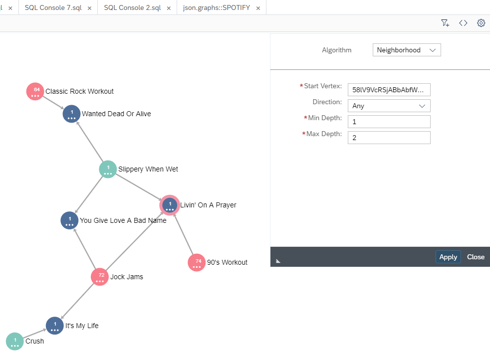
Based on the relationships we created for Spotify, track and album are one node away from artist or depth of one. Playlist would be two nodes away or depth of two. The neighbors algorithm takes the graph workspace and a starting vertex, in this example an artist id, the minimum depth as 1 and the maximum depth as 1 and the direction as “any”. The Spotify relationships are only have one direction so “ANY” and “INCOMING” will produce the same results and “OUTGOING” will produce zero results.
Using the graph workspace in Database Explorer, we can use the neighborhood algorithm to visually represent the relationships. Albums are represented in green and tracks in blue.
If we wanted to understand what playlists Bon Jovi has tracks in, we can change the maximum depth to 2.
Conclusion
We have taken semi-structured data in the form of JSON documents and transformed it into relational data in SQL views and SAP HANA calculation views. Based on the structured data, we were able to create a graph network of relationships within the Spotify data based on artists, tracks, albums, and playlists. Once the graph workspace was created, we utilized the languages of openCypher and GraphScript to query the data for analytical processing.
What's Next
Part 3 of the series discussed data ingestion option within SAP Datasphere for semi-structured data. If there is a scenario where SAP HANA Cloud is not part of the landscape but the need for graph analysis still exists, we can do the same in SAP Datasphere. Stay tuned for the next blog that covers this process.
Here are the links for the other blogs of this series
- Part 1 – Architecture
- Part 2 – Processing Semi-Structured data in SAP HANA Cloud
- Part 3 – Processing Semi-structured data in SAP Datasphere
Part 2 discussed the options of extracting, transforming, and loading JSON documents into SAP HANA Cloud.
Now that the JSON documents are loaded and stored in SAP HANA Cloud, we can further utilize the Multi-Modeling features of SAP HANA Cloud. In this part, we are going to transform the semi-structured data into structured data to be utilized by the Graph Engine to show the relationships within the Spotify data. We will create reporting scenarios using calculation views and procedures created within SAP Business Application Studio.
This blog will cover the following:
- Describe the datasets
- Modify the JSON collections
- Create Spotify relationships
- Query JSON collections to form structured SQL Views
- Form the graph tables and graph workspace
- Query on the graph workspace with different scenarios
What is SAP HANA Graph?
Refer to blog Create graphs on SAP HANA Cloud by maxime.simon that gives a great introduction to the graph capabilities of SAP HANA Cloud if you are unfamiliar.
Describe the datasets
Using the Spotify API, Get Category’s Playlists, we pulled playlist data for categories: Mood, Workout, Party and Gaming.

Get Category's Playlists API
The JSON response from the API contains the playlist id, the name and the description along with the number of tracks in each playlist.

Get Category's Playlist JSON Response
In the section, “Executing Python Scripts” in Part 2, we were able to capture all the tracks per playlist. In this scenario, we utilized the same scripts to pull all the tracks per playlist and the track audio features by using the Spotify APIs.
A new JSON collection was created for each playlist, one for all the track information and one containing the audio features for each track.

Playlist Track Information

Playlist Track Audio Features
Modify the JSON collections
In this scenario, it is necessary to update the JSON collections with identifiers which will help when creating the views and tables needed to build the graph workspace.
For the playlist category JSON collections, we will create a new identifier as category and type, nested in playlists.

Update the playlist category JSON collections

Updated playlist category JSON collections
For the track JSON collections, we will create new identifiers to help in the process of creating the graph tables. We will add three different types as dummy variables: album, artist and track. We will also add the playlist id for each track.

Update the playlist track information JSON collections

Updated playlist track information JSON collections
Create Spotify relationships
Based on the datasets, we need to determine the relationships between the core entities. From the track JSON collections, we can learn the playlist the track belongs too, details about the track, the artist of the track, the album the track is part of and the creators of the album.
The below diagram represents the relationships we will utilize for graph capabilities. Relationships in graph can be bidirectional but, in this case, we are representing in one direction.

Spotify relationship diagram
Query JSON collections to form structured SQL views
We will create views for each core entity: track, artist, album, and playlist. We will have to create individual views for each playlist, then will union all together to form a final view for each entity.
Track Views
For the tracks, we are pulling all the attributes for a track as well as the relationships with playlist, artist and album. A track can have more than one artist, therefore we unnested the artists so there may be more than one row per track to account for multiple artists.
select  "playlist_id", "type1", "type3", "track"."id" as track_id,"track"."name" as track_name, "track"."popularity" as popularity,

 "track"."duration_ms" as duration_ms, "track"."album"."id", a."id", a."name"

from "DEMOJSON"."json.synonyms::80s Party" UNNEST "track"."artists" as a 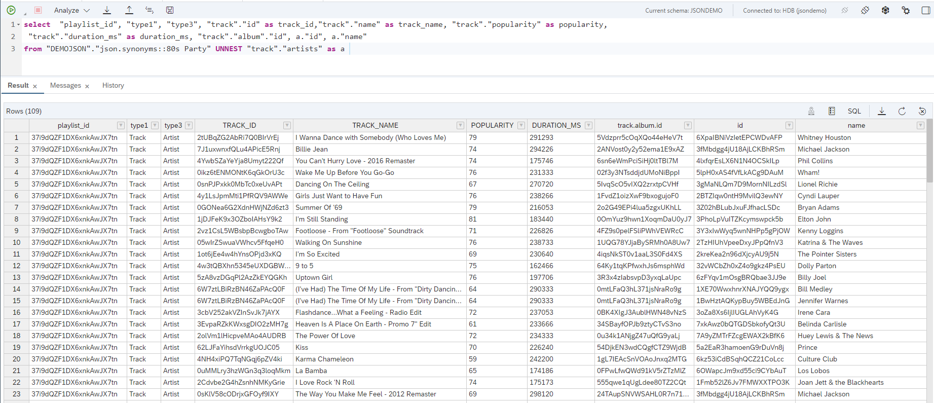
Select for track information

Track view
After the individual views were created for each playlist, we combined all the views together using a union.

Consolidated track view
Track Audio Views
For the tracks, we are also pulling audio features for the track from each playlist JSON collection.
select "id" as id, "acousticness", "danceability", "genres", "energy","key","loudness","mode","speechiness", "instrumentalness", "liveness", "valence", "tempo"

from "DEMOJSON"."json.synonyms::All The Feels_AUD"

Select for track audio features

Track audio view
After the individual views were created for each playlist, we combined all the views together using a union.

Consolidated track audio view
Track and Audio Feature View
Consolidating further, all the tracks and their audio features were combined into one view.
with x as (select  "playlist_id", "type1", "type3",  track_id, track_name,   popularity,  duration_ms, "track.album.id", "id", "name"

from "DEMOJSON"."json.Views.tracks::tracks_all"), y as (select "ID" , "acousticness", "danceability", "genres", "energy","key","loudness","mode","speechiness",

"instrumentalness", "liveness", "valence", "tempo" from "DEMOJSON"."json.Views.audio::tracks_audio_all")

select "playlist_id", "type1", "type3",  track_id, track_name,   popularity,  duration_ms, "track.album.id", "id", "name", "acousticness",

"danceability", "genres", "energy","key","loudness","mode","speechiness", "instrumentalness", "liveness", "valence", "tempo"

from x left outer join y on x.track_id = y.ID
Select for track and audio features

Track and audio features view
Playlist Views
For the playlists, we are selecting all of the attributes from each of the four JSON collections (gaming, mood, party, workout).
select "playlists"."category" as category,"playlists"."type" as type, p."id" as playlist_id, p."name" as playlist_name, p."description" as description, p."tracks"."total" as total_tracks

from "DEMOJSON"."json.synonyms::PLAYLIST_CATEGORY_GAMING" unnest "playlists"."items" as p

Select for playlist information

Playlist view
After the individual views were created, we combined all the views together using a union.
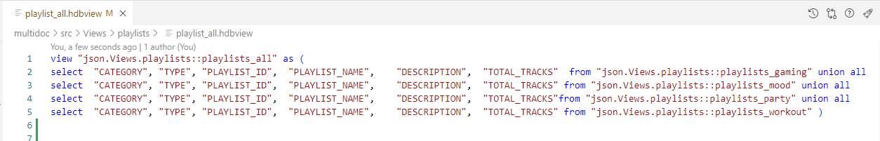
Consolidated playlist view
Album Views
For the albums, we are pulling all the attributes for each album from each playlist.
select "track"."album"."id" as album_id, "type2", "track"."album"."name" as album_name, "track"."album"."release_date" as release_date,

"track"."album"."total_tracks" as total_tracks,  a."id" as artist_id, a."name" as artist_name

from "DEMOJSON"."json.synonyms::80s Party" unnest "track"."album"."artists" as a
Select for album information

Album view
A consolidated view was created to hold all the album information from each playlist.

Consolidated album view
Form the graph tables and graph workspace
Create the nodes table
With the help of a union in a SAP HANA calculation view, we are able to combine all the entities together with each of their specific attributes.
Album
The album attributes can be found in the consolidated albums view. The columns selected from the albums view are album_id, album_name, type2 (label for Album), release_date and total tracks.

Album attributes
Playlist
The playlist attributes can be found in the consolidated playlists view. The columns selected from the playlist view are playlist_id, playlist_name, category, type (label for playlist), and total_tracks.

Playlist attributes
Track
The track attributes can be found in the consolidated track and audio view. The columns selected from the track and audio view are track_id, track_name, type1 (label for track), popularity, duration_ms, acousticness, danceability, and genres.

Track attributes
Artist
The artist attributes can be found in the consolidated track and audio view. The columns selected from the track and audio view are id, name and type3 (label for artist).

Artist attributes
A union was created to map all the separate entities and their attributes into one. Because not every entity has the same columns there will be some results with blank columns.

Union node
For the case that a song may exist in more than one playlist, we need to remove duplicates for graph to work properly as the ID of a track in the nodes table needs to be unique. A calculated column IDforRank was created specifically to partition based on ID in the rank function.

Rank logic
After the row number function generates a new column, we filter on the column to only get the top record.
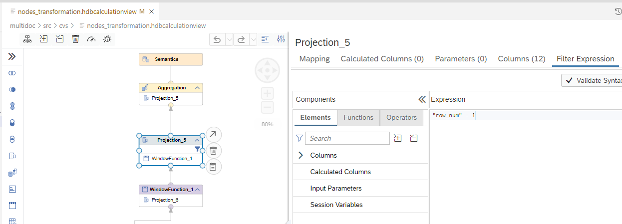
Filter out duplicates
The output of the nodes calculation view looks like this:

Data preview of nodes calculation view
Create the edges table
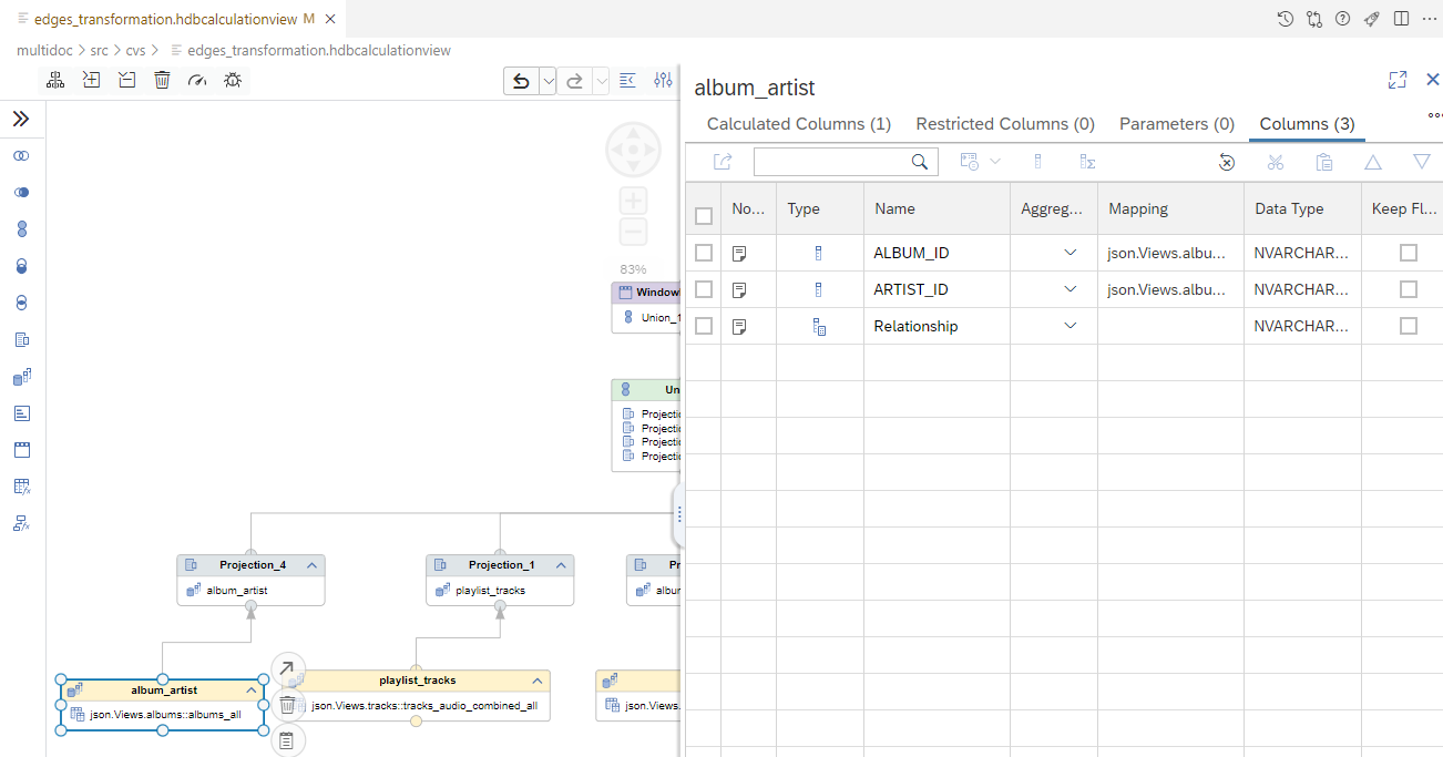
With a similar design to the nodes calculation view, the edges calculation view combines all of the entity relationships together.
Album and Artist Relationship
This relationship can be found in the consolidated albums view. The columns selected from the albums view are album_id and artist_id. A calculated column was created to define the relationship type, which in the case of album and artist is “iscreatedby”.
Album and artist IDs

Album and artist relationship
Playlist and Track Relationship
This relationship can be found in the consolidated tracks and audio view. The columns selected from the view are playlist_id and track_id. A calculated column was created to define the relationship type, which in the case of playlist and track is “contains”.

Playlist and track IDs

Playlist and track relationship
Album and Track Relationship
This relationship can be found in the consolidated tracks and audio view. The columns selected from the view are track_album_id and track_id. A calculated column was created to define the relationship type, which in the case of album and track is “contains”.

Album and track IDs

Album and track relationship
Track and Artist Relationship
This relationship can be found in the consolidated tracks and audio view. The columns selected from the view are track_id and artist_id. A calculated column was created to define the relationship type, which in the case of track and artist is “iscreatedby”.

Track and artist IDs

Track and artist relationship
A union was created to map all the separate entity relationships into one.

Union node
A rank function of row number was used to create an ID which is needed for the edges table.

Rank function
The output of the edges calculation view look like this:

Data preview of edges calculation view
Create the graph workspace
Tables, views and synonyms can be used as sources in the graph workspace. In this scenario, we created the sources to the graph workspace with calculation views. They can be used however because of the data volume, we decided to load the results of the calculation views into edges and nodes tables.
Using hdbtable database artifacts, we created the edges and nodes tables with the appropriate columns.

Edges table

Nodes table
A simple procedure was created to load the data from the calculation view into the respective tables.

Load graph tables procedure
The graph workspace was created with the edges and nodes tables with both having ID as their unique identifier.

Graph workspace

Vertices, edges, and workspaces
Query the graph workspace with different scenarios
OpenCypher is a declarative graph query language for pattern matching. In SAP HANA, we can use openCpher directly in SQL querying on the graph workspace we created.
If we want to understand how many tracks for a specific genre exist in each playlist and category, we can use the OPENCYPHER_TABLE SQL function that enables the embedding of an openCypher query in an SQL query.
SELECT DISTINCT *

    FROM OPENCYPHER_TABLE (

         GRAPH WORKSPACE "DEMOJSON"."json.graphs::SPOTIFY"

         QUERY '

          MATCH   (a)-[e]-(b)

            WHERE   a.GENRE contains ''country''

            and b.TYPE = ''Playlist''

             RETURN  b.PLAYLISTCATEGORY as playlist_category,

            b.NAME as playlist_name, count(a.ID) as number_of_tracks'

    )

Result of openCypher query
We can visually represent the results of the openCypher MATCH operation in Database Explorer. Playlists are represented in pink and tracks represented in blue.

Cypher in Database Explorer
Business users might not understand the openCypher language. We can create table functions which can be used within SAP HANA calculation views which can be exposed to the business users.
The table function would have the input parameter “genre” and execute the openCypher SQL using OPENCYPER_TABLE.

Table function with openCypher
This table function will be an input into the calculation view that will have the same input parameter which is mapped to the table function.

Table function as input for calculation view

Input parameter mapped to table function
The business user can run a select statement on the calculation view with the genre of their choice.
SELECT

	"playlist_category",

	"playlist_name",

    "number_of_tracks"

FROM "DEMOJSON"."json.cvs::genres_tbf"

	(placeholder."$$IP_Genre$$"=>'country')

order by "number_of_tracks" desc
Select on calculation view
GraphScript is an imperative programming language with built in functions that can be integrated into SQL-based data processing. Graphscript can be used within stored procedures, anonymous blocks, and table functions.
We can use the built-in GraphScript function in an SAP HANA stored procedure to identify all of a artists tracks and albums based on the graph workspace.

Stored procedure with neighbors algorithm
Based on the relationships we created for Spotify, track and album are one node away from artist or depth of one. Playlist would be two nodes away or depth of two. The neighbors algorithm takes the graph workspace and a starting vertex, in this example an artist id, the minimum depth as 1 and the maximum depth as 1 and the direction as “any”. The Spotify relationships are only have one direction so “ANY” and “INCOMING” will produce the same results and “OUTGOING” will produce zero results.
CALL "DEMOJSON"."json.procedures::NEIGHBORS_P"(

i_startVertex => '58lV9VcRSjABbAbfWS6skp',

i_minDepth => 1,

i_maxDepth => 1,

i_dir => 'ANY',

o_vertices => ?,

o_verticesCount => ?,

o_edges => ?);
Results of procedure call
Using the graph workspace in Database Explorer, we can use the neighborhood algorithm to visually represent the relationships. Albums are represented in green and tracks in blue.

Graph workspace neighborhood algorithm
If we wanted to understand what playlists Bon Jovi has tracks in, we can change the maximum depth to 2.

Result of procedure call with max depth of 2
Graph workspace neighborhood algorithm with max depth of 2
Conclusion
We have taken semi-structured data in the form of JSON documents and transformed it into relational data in SQL views and SAP HANA calculation views. Based on the structured data, we were able to create a graph network of relationships within the Spotify data based on artists, tracks, albums, and playlists. Once the graph workspace was created, we utilized the languages of openCypher and GraphScript to query the data for analytical processing.
What's Next
Part 3 of the series discussed data ingestion option within SAP Datasphere for semi-structured data. If there is a scenario where SAP HANA Cloud is not part of the landscape but the need for graph analysis still exists, we can do the same in SAP Datasphere. Stay tuned for the next blog that covers this process.
Labels:
You must be a registered user to add a comment. If you've already registered, sign in. Otherwise, register and sign in.
Labels in this area
-
ABAP CDS Views - CDC (Change Data Capture)
2 -
AI
1 -
Analyze Workload Data
1 -
BTP
1 -
Business and IT Integration
2 -
Business application stu
1 -
Business Technology Platform
1 -
Business Trends
1,658 -
Business Trends
92 -
CAP
1 -
cf
1 -
Cloud Foundry
1 -
Confluent
1 -
Customer COE Basics and Fundamentals
1 -
Customer COE Latest and Greatest
3 -
Customer Data Browser app
1 -
Data Analysis Tool
1 -
data migration
1 -
data transfer
1 -
Datasphere
2 -
Event Information
1,400 -
Event Information
66 -
Expert
1 -
Expert Insights
177 -
Expert Insights
295 -
General
1 -
Google cloud
1 -
Google Next'24
1 -
Kafka
1 -
Life at SAP
780 -
Life at SAP
13 -
Migrate your Data App
1 -
MTA
1 -
Network Performance Analysis
1 -
NodeJS
1 -
PDF
1 -
POC
1 -
Product Updates
4,577 -
Product Updates
341 -
Replication Flow
1 -
RisewithSAP
1 -
SAP BTP
1 -
SAP BTP Cloud Foundry
1 -
SAP Cloud ALM
1 -
SAP Cloud Application Programming Model
1 -
SAP Datasphere
2 -
SAP S4HANA Cloud
1 -
SAP S4HANA Migration Cockpit
1 -
Technology Updates
6,873 -
Technology Updates
419 -
Workload Fluctuations
1
Related Content
- Exploring Integration Options in SAP Datasphere with the focus on using SAP extractors - Part II in Technology Blogs by SAP
- New Machine Learning features in SAP HANA Cloud in Technology Blogs by SAP
- 10+ ways to reshape your SAP landscape with SAP Business Technology Platform – Blog 4 in Technology Blogs by SAP
- Top Picks: Innovations Highlights from SAP Business Technology Platform (Q1/2024) in Technology Blogs by SAP
- Enhanced Data Analysis of Fitness Data using HANA Vector Engine, Datasphere and SAP Analytics Cloud in Technology Blogs by SAP
Top kudoed authors
| User | Count |
|---|---|
| 35 | |
| 25 | |
| 17 | |
| 13 | |
| 8 | |
| 7 | |
| 6 | |
| 6 | |
| 6 | |
| 6 |