
- SAP Community
- Products and Technology
- Technology
- Technology Blogs by SAP
- Harnessing Multi-Model Capabilities with Spotify –...
Technology Blogs by SAP
Learn how to extend and personalize SAP applications. Follow the SAP technology blog for insights into SAP BTP, ABAP, SAP Analytics Cloud, SAP HANA, and more.
Turn on suggestions
Auto-suggest helps you quickly narrow down your search results by suggesting possible matches as you type.
Showing results for
Product and Topic Expert
Options
- Subscribe to RSS Feed
- Mark as New
- Mark as Read
- Bookmark
- Subscribe
- Printer Friendly Page
- Report Inappropriate Content
03-31-2023
3:42 AM
In the first two blogs of this series focusing on Architecture and hands-on for the Document Store, we discussed the deployment options in SAP HANA Cloud. In this part of the blog series, we will focus on deployment options on SAP Datasphere and will be covering the following topics related to Spotify data:
Here are the links for the other blogs of this series
Part 1 - Architecture
Part 2 - Processing Semi-Structured data in SAP HANA Cloud
Part 4 – Processing Semi-Structured data in SAP HANA Cloud & creating graph networks
Part 5 – Building Intelligent Data Apps based on Spotify Datasets
Part 6 – Visualization
In the previous blogs related to architecture and SAP HANA Cloud hands-on, we discussed different scenarios of data ingestion and hands-on for SAP HANA Cloud. Let’s proceed with handling the semi-structured data in SAP Datasphere.
Well, the document store is not enabled in SAP Datasphere. There is a difference when considering SAP HANA Cloud as a data mart compared to SAP Datasphere. With the foundation of a business data fabric architecture, SAP Datasphere enables self-service data access seamlessly. To process semi-structured data within SAP Datasphere, let me explain it with a decision tree. Also, this decision tree is my perspective on how you process APIs/semi-structured data from SaaS solutions or cloud storage.
One should look for standard SAP/ Non-SAP/Open or partner connectors to ingest semi-structured data from SaaS solutions. Let’s consider a few scenarios to go through the decision tree. The standard connectors are available for S/4HANA Cloud, Fieldglass, or SAP SuccessFactors if you want to federate or replicate data from our SAP Cloud Solutions. Say if you are looking for Ariba Spend Analytics, we do not have a standard connector as per our current documentation. SAP suggests using an ETL partner, and if you look for partner connectors, Precog provides connectors for multiple connectors for Ariba, say Spend Analysis or Operational Procurement. I would also suggest you explore our Discovery Center to see if any missions would help you adopt the solution if you already have BTP entitlements for the Integration suite. Take the same example for Ariba, and there is a Discovery Mission that helps you with a step-by-step process for extracting Ariba Spend data using Integration Suite.
The same decision process applies to non-SAP sources too. Still, you will also see the additional option to explore Open connectors if you plan to ingest data from Web-based analytics or social media. And suppose you do not find any connectors after exploring all the possibilities. In that case, you can follow the same approach we are about to do with ingesting Spotify response into SAP Datasphere using Open SQL schemas.
With the Spotify example, I am sharing the python scripts, which you could test from your laptops/virtual machines. Still, there should be some Data Orchestration tool or compute, such as SAP Data Intelligence Cloud or SAP Kyma, to execute the scripts in real-life scenarios. In upcoming weeks, I will share an interesting example using SAP Kyma for bulk data load from Databricks to SAP HANA Cloud or Data Lake. Now let’s go back to Spotify. 😊
We have already shared this in the architecture blog. Still, I want to emphasize again that when we ingest data into Open SQL schemas, we connect to the SAP HANA Cloud tenant of SAP Datasphere, which is why you see the same in the architecture. Open SQL schema is Space specific, and you will be reading the ingested data from Datasphere Space for SAP Analytics Cloud reporting scenarios. Please refer to his blog for more details about how these all work.
For SAP Datasphere, I am considering two approaches to ingest data from Spotify APIs:
Ideally, preserving the JSON response, as mentioned in option 1, is better than extracting the information as needed. If you are sure only specific attributes are required, you can choose option 2.
Let’s discuss the dataflow 1 -> 2 -> 3 -> 5 and the relevant code in detail. Here are the steps to be followed:
As mentioned in the pre-requisite, I assume you know the Open SQL schema concept. Navigate to your Space and create a Database user[1] with Read/Write access to Space schema and HDI consumption. Once the user is created, select the Database User Name[2] and navigate to the Database explorer [3], as shown below.
Once you are in SAP HANA Database explorer, you are connected to the SAP HANA Cloud tenant of the SAP Datasphere. As mentioned in the steps, let’s create a table to ingest the JSON response. Like how we stored the Country Name and the JSON response as a document in blog two scenarios, we are following the same process but keeping it as NCLOB. My table name is “CL4”; the JSON response will be stored in the column TOPTRACKS as NCLOB.
Now that the table is created let’s execute the python script. As discussed in blog 2, I hope you have MS Visual Studio, Google Colabs, or any python environment for running the scripts.
Here is the script, and please replace all input variables with your Spotify and Open SQL schema credentials.
The script is almost the same as we used for the document store scenario, but it starts deviating from line 27. While storing as a JSON document in blog2, we insert the JSON response from line 26 as JSON collection. If you try to do the same in SAP Datasphere, you will notice the error “No active JSON Document Store found or enabled in your landscape.” Instead, we dump the JSON response as a string(JSON formatted string), as shown in line 27. And in line 28, we call the insert function to ingest the response into the Open SQL schema.
In the insert_json_hcdb function, we provide the connection details of the Open SQL schema (lines 33-38). In lines 39-40, we use the datetime function to append the date to the country name so that the files are evident in case you plan to schedule weekly or daily. Finally, we insert the JSON file stored as text and the country name to the table CL4. In the case of the Document store scenario, we utilized the class hana_ml, and schema and collection ingestion were dynamic. But it’s a different case when we use the hdbcli package.
Now the exciting part is to explore the ingested data from SAP HANA Database Explorer. If I execute the select on table CL4, you will notice the country name with the date appended followed by JSON response in the column “TOPTRACKS”
If you explore using the JSON viewer, it will be the similar response we explored in blog 2. We should see 50 JSON responses for the top 50 songs in the USA for a specific week.
We are still developing from the SAP HANA Cloud tenant of SAP Datasphere, which allows us to use SAP HANA Cloud SQL functions. In this scenario, we will be using the JSON_TABLE function. Here is the SQL function that is executed on column TOPTRACKS
And here is the navigation path for the same
So in the SQL function, we have mentioned the statement NESTED PATH and provided the navigation path.
Now we have the JSON response as SQL for the column tracks. But we also need the column COUNTRY to group all the tracks by country. So here we go,
So, we have all 50 songs grouped by country, TOPUSA, this week. But we have 50 JSON responses in the TOPTRACKS, and the SQL functions we executed resulted in 56 records. We have more than one artist for specific tracks and additional rows with different artists.
This is when I tell you to take a chill pill 😊called the string aggregate function.
String aggregate concatenates the artist’s name with a separator when we order the results by Song. And here we go(In actual use cases, please use a valid separator 😊),
And so, we are back with 50 records as relational similar to 50 JSON responses. Aren’t these functions cool? This is how you convert the JSON responses as relational in SAP Datasphere.
I have explained how you would normalize the data within Datasphere for the Spotify Playlist scenario. For Audio Features API, we have already shared the script in blog2. Now we will adjust the code the same way we did previously. Kindly modify the lines where you must add credentials and Open SQL schema access inputs.
Again, we introduced the JSON.dumps at line 43 to return the audio features as JSON formatted string. In line 47, we call the insert function to ingest the JSON formatted string to SAP Datasphere. And we access the SAP Datasphere through database access (Open SQL schema).
And in the insert function, we again provide the table name (CL5 in my case) and give the inputs as country name (USA + DateTime added to the name of country) and the formatted JSON response as a string.
Here is the structure of the table CL5, as part of the Open SQL schema
And you can validate the data that we ingested using Python.
Let’s check the response using JSON viewer, and we are lucky that Audio features do not have the same nested structure as playlist response.
Since there are no nested structures, we can provide the root path of the response as ‘$’ and directly extract the attributes using the SQL function as below:
Woohoo! We could ingest data as JSON and query using JSON to SQL functions.
This is, again, an optional way of ingesting data into SAP Datasphere. If you are not interested in this option, you can skip this section and navigate to the Data Builder section to build views and consumption models.
In this option, we will rely on python capabilities to normalize the JSON response and ingest it as relational data into Open SQL schema. If nothing works, we can still ingest data using the SQL layer. So, in this scenario, we execute a similar script as other scenarios (well, not so similar) but will rely on the pandas library json_normalize function to normalize the response from Spotify. If there are deep nested structures within the response, then we have to use the explode function to list the data like rows and normalize the data.
Here is the script for the same.
The script is the same till line 40, extracting the JSON response from items. Since we cannot store it as a collection nor use the JSON functions from SAP HANA Cloud, we normalize the JSON response at line 42 using json_normalize. When we try to flatten the JSON response the first time, we know all the attributes except the artists’ info will be managed successfully. So we have to isolate the artist column, execute the explode function mentioned before and then concatenate the response with other columns.
Say you comment out the rest of the code after line 42 and print the response of the json_normalize, just focusing on two attributes album name and artists info. You can see the Album name is not nested while the artist’s info is, so we have to normalize the artist’s information again.
If you want to learn how this works, print the response after lines 42, 44, 46,51 & 55. Adjust the code and execute the print function as separate scenarios, and it would be much easier to understand. Assuming all the normalization was successful, you should see the entries in the table countall555 (Again, don’t ask me why I chose this name).
Again, you can execute the string aggregate function to aggregate it back to 50 JSON responses, as discussed before. Now, try the same approach for Audio features and see if it works. And we have gone through 2 different options for Data Ingestion using Open SQL schema.
Now that we have investigated options for ingesting data into SAP Datasphere let’s focus on consuming the data in the data builder layer and exposing it to SAP/Non-SAP reporting tools. You can consider this section follow-up steps for Data Ingestion Option 1, i.e., Store JSON as a string and normalize internally.
We know the string aggregate function was executed on top of the JSON string.
Now we create a view directly based on the previous SQL statement. And we follow the same approach for Audio features API too. Kindly execute the following statements from Database explorer.
Once you have executed it, you should see the view from DB explorer.
You will consume these views in Data builder for building consumption views. We must create these views here rather than directly in SAP Datasphere because SQL view builder prevents us from using JSON to SQL functions.
Based on the artifacts CL4_V(Playlist Data) & CL5_V(Audio Features), I created views TOPTRACKS and AUDIOFEATURES. In the view AUDIOFEATURES, I made an association with TOPTRACKS. So, the final consumption view(SPOTIFYTRACKS) will be an inner join between the two views, as seen below.
And this will be the join condition you will use between these two views.
You can extend this view as the new Analytic model that could be used as a consumption view for SAP Analytics cloud or Microsoft Power BI.
Yes, we have done with all developments based on SAP HANA Cloud(Part2) or SAP Datasphere. We will move on with Visualizations in the next blog. And I promise to keep it short for the next one, and the viz do the talking!
Visualizations on SAP Analytics Cloud based on R computations [Danceability & Speechiness Distribution]
What if we could slice and dice reporting based on images? Here are the 500 songs collaged for ten countries for a specific week in Microsoft Power BI. Feeling it? 😉
And here are the top 50 songs in the US & India based on Speechiness and Popularity for a particular week! Still feeling it? 😊
Thanks for reading till the end! And, of course, there will be follow-up blogs covering other multi-model capabilities based on different Spotify API scenarios. Please do share your feedback regarding the scenarios and approach we took. And if you have issues accessing git repositories or problems with the code, let us know. Happy learning!
- Data Ingestion Options within SAP Datasphere for semi-structured data
- Revisit Architecture specific to SAP Datasphere for processing JSON data
- Data Ingestion Options Hands-on for Option 1 [Save JSON and normalize internally]
- Data Ingestion Options Hands-on for Option 2 [Normalize externally and save as relational]
- Use Data builder to build consumption models [Based on Point 3 – Data Ingestion Option 1]
- Follow-up blogs as part of this series
Here are the links for the other blogs of this series
Part 1 - Architecture
Part 2 - Processing Semi-Structured data in SAP HANA Cloud
Part 4 – Processing Semi-Structured data in SAP HANA Cloud & creating graph networks
Part 5 – Building Intelligent Data Apps based on Spotify Datasets
Part 6 – Visualization
Data Ingestion options for SAP Datasphere
In the previous blogs related to architecture and SAP HANA Cloud hands-on, we discussed different scenarios of data ingestion and hands-on for SAP HANA Cloud. Let’s proceed with handling the semi-structured data in SAP Datasphere.
What happened to Document Store in SAP Datasphere?
Well, the document store is not enabled in SAP Datasphere. There is a difference when considering SAP HANA Cloud as a data mart compared to SAP Datasphere. With the foundation of a business data fabric architecture, SAP Datasphere enables self-service data access seamlessly. To process semi-structured data within SAP Datasphere, let me explain it with a decision tree. Also, this decision tree is my perspective on how you process APIs/semi-structured data from SaaS solutions or cloud storage.

SAP Sources

Non-SAP Sources
One should look for standard SAP/ Non-SAP/Open or partner connectors to ingest semi-structured data from SaaS solutions. Let’s consider a few scenarios to go through the decision tree. The standard connectors are available for S/4HANA Cloud, Fieldglass, or SAP SuccessFactors if you want to federate or replicate data from our SAP Cloud Solutions. Say if you are looking for Ariba Spend Analytics, we do not have a standard connector as per our current documentation. SAP suggests using an ETL partner, and if you look for partner connectors, Precog provides connectors for multiple connectors for Ariba, say Spend Analysis or Operational Procurement. I would also suggest you explore our Discovery Center to see if any missions would help you adopt the solution if you already have BTP entitlements for the Integration suite. Take the same example for Ariba, and there is a Discovery Mission that helps you with a step-by-step process for extracting Ariba Spend data using Integration Suite.
The same decision process applies to non-SAP sources too. Still, you will also see the additional option to explore Open connectors if you plan to ingest data from Web-based analytics or social media. And suppose you do not find any connectors after exploring all the possibilities. In that case, you can follow the same approach we are about to do with ingesting Spotify response into SAP Datasphere using Open SQL schemas.

With the Spotify example, I am sharing the python scripts, which you could test from your laptops/virtual machines. Still, there should be some Data Orchestration tool or compute, such as SAP Data Intelligence Cloud or SAP Kyma, to execute the scripts in real-life scenarios. In upcoming weeks, I will share an interesting example using SAP Kyma for bulk data load from Databricks to SAP HANA Cloud or Data Lake. Now let’s go back to Spotify. 😊
The Interim

Now the Architecture – SAP Datasphere
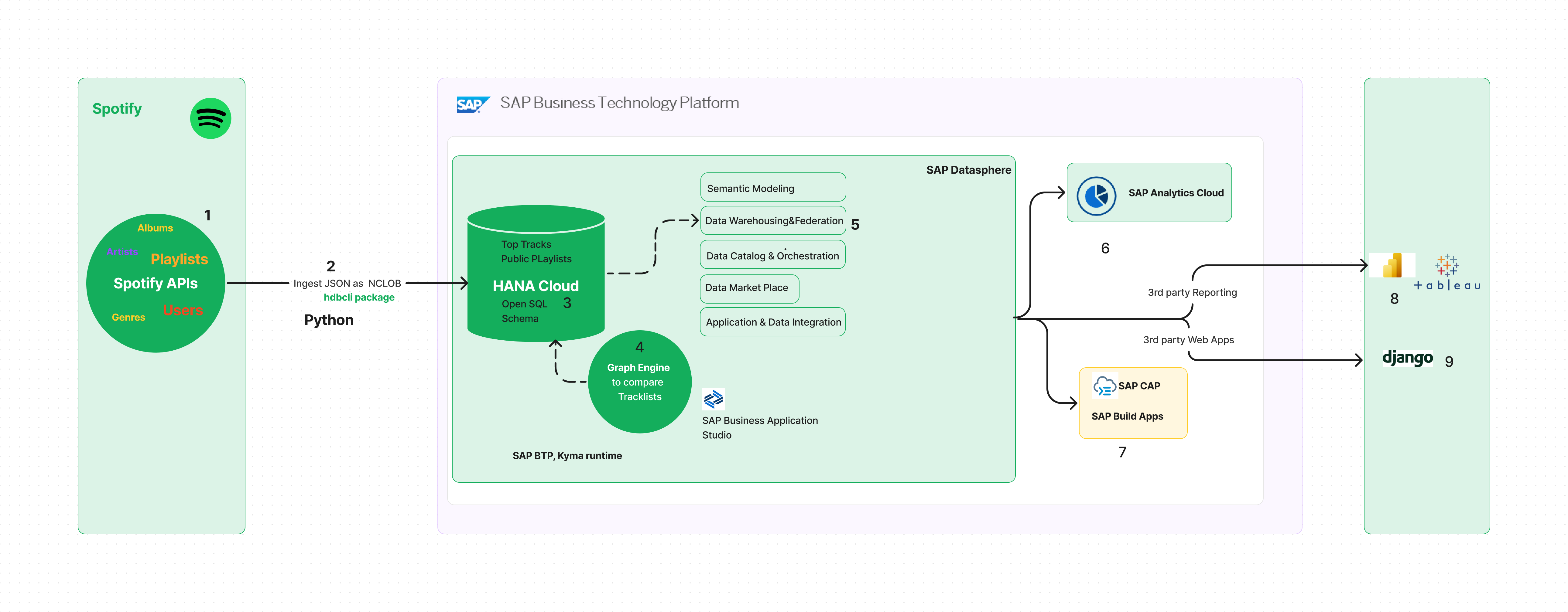
We have already shared this in the architecture blog. Still, I want to emphasize again that when we ingest data into Open SQL schemas, we connect to the SAP HANA Cloud tenant of SAP Datasphere, which is why you see the same in the architecture. Open SQL schema is Space specific, and you will be reading the ingested data from Datasphere Space for SAP Analytics Cloud reporting scenarios. Please refer to his blog for more details about how these all work.

For SAP Datasphere, I am considering two approaches to ingest data from Spotify APIs:
- Ingest the JSON response as a large object [2] into Open SQL schema and use SAP HANA Cloud SQL functions JSON_TABLE to normalize the JSON response. The Spotify response is ingested into SAP HANA Cloud using the package hdbcli.
- Normalize the JSON response externally [2.2] and ingest the data as relational into Open SQL schema. The Spotify response is ingested into SAP HANA Cloud using the package hana_ml.
Ideally, preserving the JSON response, as mentioned in option 1, is better than extracting the information as needed. If you are sure only specific attributes are required, you can choose option 2.
Data Ingestion – Option 1 - Save the Response and Normalize later
Pre-Requisite:
- You know the Open SQL schema concept and access the same using DB Explorer.
- Since we use the hdbcli package, the table must be created before executing the script. Of course, you can create it as part of the script before data ingestion.
Approach 1 - Normalize Internally
Let’s discuss the dataflow 1 -> 2 -> 3 -> 5 and the relevant code in detail. Here are the steps to be followed:
- Navigate to your Space in SAP Datasphere, and create a Database User that allows you to read and write into Open SQL schema with external tools.
- Connect to the Open SQL schema with Database Explorer.
- Create a table with two columns Country Name (type String) and Track response (type NCLOB)
- Execute Python script to ingest the JSON response as a large object in the newly created table.
- Execute SAP HANA Cloud SQL functions to normalize the data stored in the table.
- Execute Procedure to normalize all JSON responses and store them as table
Database user Creation [Open SQL Schema]
As mentioned in the pre-requisite, I assume you know the Open SQL schema concept. Navigate to your Space and create a Database user[1] with Read/Write access to Space schema and HDI consumption. Once the user is created, select the Database User Name[2] and navigate to the Database explorer [3], as shown below.

Once you are in SAP HANA Database explorer, you are connected to the SAP HANA Cloud tenant of the SAP Datasphere. As mentioned in the steps, let’s create a table to ingest the JSON response. Like how we stored the Country Name and the JSON response as a document in blog two scenarios, we are following the same process but keeping it as NCLOB. My table name is “CL4”; the JSON response will be stored in the column TOPTRACKS as NCLOB.
CREATE TABLE CL4 (COUNTRY NVARCHAR(20), TOPTRACKS NCLOB);
Now that the table is created let’s execute the python script. As discussed in blog 2, I hope you have MS Visual Studio, Google Colabs, or any python environment for running the scripts.
Ingesting Playlist Response into SAP Datasphere
Here is the script, and please replace all input variables with your Spotify and Open SQL schema credentials.
import pandas as pd

import spotipy

import spotipy.util as util

import json

from hdbcli import dbapi

from datetime import datetime

client_id = "XXXXXXXXXXXXXXXXXXXXXXXX"  #Your Spotify Client ID -Refer Blog2  of this series

client_secret = "XXXXXXXXXXXXXXXXXXXXXXXXXXX" #Your Spotify Secret Key -Refer Blog2 of this series

redirect_uri = "http://localhost:8888/callback"

username = "XXXXXX"  #Your Spotify Username

scope = "user-library-read user-top-read playlist-read-private"

# Get the access token

token = util.prompt_for_user_token(

    username, scope, client_id, client_secret, redirect_uri)

# Create the Spotify client

sp = spotipy.Spotify(auth=token)

#Process all tracks and items of a specific playlist

def get_top2022_playllst(playlistid, country):

    playlist2022 = playlistid

    collname   = country

    toptracks1 = sp.user_playlist(username, playlist2022)

    tracks1 = toptracks1["tracks"]

    toptracks = tracks1["items"]

    t2  = json.dumps(toptracks)    #here we store the json information as a text file in t2

    finaljson = insert_json_hcdb(t2,collname) #call the insert function

    print(collname + " tracks has been succesfully inserted")

#Collect all the playlist data and insert it into HANA Cloud tenant of Datasphere as NCLOB

def insert_json_hcdb(t3, country1):

    conn = dbapi.connect (address= 'XXXXXX',  # Provide your OpenSQL Host here

                      port= '443',

                      user= 'XXXXXXX',  # Provide your OpenSQL container Username here

                      password= 'XXXXXX',  # Provide your OpenSQL contianer password here

                      encrypt=True

                     ) #establish open SQL schema access

    get = datetime.now()

    cntdaily = country1 + str(get.day)+ str(get.month)+str(get.year)   #add datetime to filename country

    sql = 'INSERT INTO CL4 (COUNTRY, TOPTRACKS) VALUES (?,?)'

    cursor = conn.cursor()

    cursor.execute(sql,(cntdaily,t3))

    cursor.close()

    conn.close()

    return country1

# Get all top playlist from different countries

playlist2022 = get_top2022_playllst('37i9dQZEVXbLp5XoPON0wI','USA')

#Add additional playlists as needed
The script is almost the same as we used for the document store scenario, but it starts deviating from line 27. While storing as a JSON document in blog2, we insert the JSON response from line 26 as JSON collection. If you try to do the same in SAP Datasphere, you will notice the error “No active JSON Document Store found or enabled in your landscape.” Instead, we dump the JSON response as a string(JSON formatted string), as shown in line 27. And in line 28, we call the insert function to ingest the response into the Open SQL schema.

In the insert_json_hcdb function, we provide the connection details of the Open SQL schema (lines 33-38). In lines 39-40, we use the datetime function to append the date to the country name so that the files are evident in case you plan to schedule weekly or daily. Finally, we insert the JSON file stored as text and the country name to the table CL4. In the case of the Document store scenario, we utilized the class hana_ml, and schema and collection ingestion were dynamic. But it’s a different case when we use the hdbcli package.

Now the exciting part is to explore the ingested data from SAP HANA Database Explorer. If I execute the select on table CL4, you will notice the country name with the date appended followed by JSON response in the column “TOPTRACKS”

If you explore using the JSON viewer, it will be the similar response we explored in blog 2. We should see 50 JSON responses for the top 50 songs in the USA for a specific week.

How do we query this if we do not have a Document store in SAP Datasphere?
We are still developing from the SAP HANA Cloud tenant of SAP Datasphere, which allows us to use SAP HANA Cloud SQL functions. In this scenario, we will be using the JSON_TABLE function. Here is the SQL function that is executed on column TOPTRACKS
SELECT JT.* FROM JSON_TABLE("CL4"."TOPTRACKS", '$.track'

COLUMNS

    (


        Albname  NVARCHAR(60) PATH '$.album.name',

        Song     NVARCHAR(60) PATH  '$.name',

        NESTED PATH '$.album.artists'

        COLUMNS

        (ARTISTNAME NVARCHAR(100) PATH '$.name'

        )

     ))  AS JT;

And here is the navigation path for the same

So in the SQL function, we have mentioned the statement NESTED PATH and provided the navigation path.

Now we have the JSON response as SQL for the column tracks. But we also need the column COUNTRY to group all the tracks by country. So here we go,
SELECT COUNTRY, Albname, SONG , ARTISTNAME FROM CL4 , JSON_TABLE("CL4"."TOPTRACKS", '$.track'

COLUMNS

    (


        Albname  NVARCHAR(60) PATH '$.album.name',

        Song     NVARCHAR(60) PATH  '$.name',

        NESTED PATH '$.album.artists'

        COLUMNS

        (ARTISTNAME NVARCHAR(100) PATH '$.name'

        )

     ))

     ORDER BY ALBNAME;
So, we have all 50 songs grouped by country, TOPUSA, this week. But we have 50 JSON responses in the TOPTRACKS, and the SQL functions we executed resulted in 56 records. We have more than one artist for specific tracks and additional rows with different artists.

How do we adjust the duplicate records?
This is when I tell you to take a chill pill 😊called the string aggregate function.

String aggregate concatenates the artist’s name with a separator when we order the results by Song. And here we go(In actual use cases, please use a valid separator 😊),
SELECT COUNTRY, Albname,SONG, STRING_AGG(ARTISTNAME,';' ORDER BY SONG) AS ARTISTS FROM

(SELECT COUNTRY, Albname, SONG , ARTISTNAME FROM CL4 , JSON_TABLE("CL4"."TOPTRACKS", '$.track'

COLUMNS

    (


        Albname  NVARCHAR(60) PATH '$.album.name',

        Song     NVARCHAR(60) PATH  '$.name',

        NESTED PATH '$.album.artists'

        COLUMNS

        (ARTISTNAME NVARCHAR(100) PATH '$.name'

        )

      -- img  NVARCHAR(600) PATH  '$.album.images.url',


        --durationms  integer   PATH  '$.duration_ms'


     ))

     ORDER BY ALBNAME)

     GROUP BY

     COUNTRY, Albname, SONG

And so, we are back with 50 records as relational similar to 50 JSON responses. Aren’t these functions cool? This is how you convert the JSON responses as relational in SAP Datasphere.
Ingesting Audio Features Response into SAP Datasphere
I have explained how you would normalize the data within Datasphere for the Spotify Playlist scenario. For Audio Features API, we have already shared the script in blog2. Now we will adjust the code the same way we did previously. Kindly modify the lines where you must add credentials and Open SQL schema access inputs.
import pandas as pd

import spotipy

import spotipy.util as util

import json

from hdbcli import dbapi

from datetime import datetime

client_id = "XXXXXXXXXXXXXXXXXXXXXX"  #Provide your Spotify Client ID

client_secret = "XXXXXXXXXXXXXXXXXXXXX" #Provide your Spotify secret keys

redirect_uri = "http://localhost:8888/callback"

username = "XXXXXXXXXX"  #Provide your Spotify Username

scope = "user-library-read user-top-read playlist-read-private"

# Get the access token

token = util.prompt_for_user_token(

    username, scope, client_id, client_secret, redirect_uri)

# Create the Spotify client

sp = spotipy.Spotify(auth=token)

#Process all tracks and items of a specific playlist

def get_top2022_playllst(playlistid, country):

    playlist2022 = playlistid

    collname   = country

    toptracks1 = sp.user_playlist(username, playlist2022)

    tracks1 = toptracks1["tracks"]

    toptracks = tracks1["items"]

    track_ids = []

    track_names = []

    track_artists = []

    for i in range(0, len(toptracks)):

        if toptracks[i]['track']['id'] != None:

            track_ids.append(toptracks[i]['track']['id'])

            track_names.append(toptracks[i]['track']['name'])

            track_artists.append(toptracks[i]['track']['artists'])

        features = []

    for i in range(0,len(track_ids)):

        audio_features = sp.audio_features(track_ids[i])[0]

        track_popularity = {'popularity': sp.track(track_ids[i])['popularity']}

        genre = {'genres': sp.artist(track_artists[i][0]['uri'])['genres']}

        audio_features = dict(audio_features, **track_popularity, **genre)

        features.append(audio_features)

        t2  = json.dumps(features)

        #print(t2)


    #Call the insert function now

    finaljson = insert_json_hcdb(t2,country)

    print(country + " tracks has been succesfully inserted")

#Collect all the playlist data and insert it into HANA Cloud as Collection

def insert_json_hcdb(audio_features1, country1):

    conn = dbapi.connect (address='XXXXXXXXXXXXXXXXXXXXX',  # Provide your OpenSQL Host here

                      port= '443',

                      user='XXXXXXXXXXXXXXXX',  # Provide your OpenSQL container Username here

                      password='XXXXXXXXXXXXXXXXXXXXX',  # Provide your OpenSQL container password here

                      encrypt=True

                     ) #establish open SQL schema access

    get = datetime.now()

    cntdaily = country1 + str(get.day)+ str(get.month)+str(get.year)   #add datetime to filename country

    sql = 'INSERT INTO CL5 (COUNTRY, AUDIOFEATURES) VALUES (?,?)'

    cursor = conn.cursor()

    cursor.execute(sql,(cntdaily,audio_features1))

    cursor.close()

    conn.close()

    return country1

# Get all top playlist from different countries

playlist2022 = get_top2022_playllst('37i9dQZEVXbLp5XoPON0wI','USA')
Again, we introduced the JSON.dumps at line 43 to return the audio features as JSON formatted string. In line 47, we call the insert function to ingest the JSON formatted string to SAP Datasphere. And we access the SAP Datasphere through database access (Open SQL schema).

And in the insert function, we again provide the table name (CL5 in my case) and give the inputs as country name (USA + DateTime added to the name of country) and the formatted JSON response as a string.

Here is the structure of the table CL5, as part of the Open SQL schema

And you can validate the data that we ingested using Python.

Let’s check the response using JSON viewer, and we are lucky that Audio features do not have the same nested structure as playlist response.

Since there are no nested structures, we can provide the root path of the response as ‘$’ and directly extract the attributes using the SQL function as below:
SELECT COUNTRY, ID, DANCEABILITY, SPEECHINESS, ENERGY, POPULARITY, LIVENESS  FROM "CL5",JSON_TABLE("CL5"."AUDIOFEATURES", '$'

COLUMNS

    (   ID  NVARCHAR(60) PATH '$.id',

        DANCEABILITY float PATH '$.danceability',

        SPEECHINESS  float PATH '$.speechiness',

        ENERGY  float PATH '$.energy',

        POPULARITY  integer PATH '$.popularity',

        LIVENESS  float PATH '$.liveness'

       ))

Woohoo! We could ingest data as JSON and query using JSON to SQL functions.
Data Ingestion – Option 2 - Normalize the Response Externally (Optional)
This is, again, an optional way of ingesting data into SAP Datasphere. If you are not interested in this option, you can skip this section and navigate to the Data Builder section to build views and consumption models.
Pre-Requisite:
- You know the Open SQL schema concept and access the same using DB Explorer.
In this option, we will rely on python capabilities to normalize the JSON response and ingest it as relational data into Open SQL schema. If nothing works, we can still ingest data using the SQL layer. So, in this scenario, we execute a similar script as other scenarios (well, not so similar) but will rely on the pandas library json_normalize function to normalize the response from Spotify. If there are deep nested structures within the response, then we have to use the explode function to list the data like rows and normalize the data.

Here is the script for the same.
import pandas as pd

#from pandas.io.json import json_normalize

import spotipy

import spotipy.util as util

import json

import hana_ml

from hana_ml.docstore import create_collection_from_elements as jsoncollection

from hana_ml import dataframe as dframe

import pyhdb

from hdbcli import dbapi

from datetime import datetime

pd.set_option('display.max_columns', None)

client_id = "XXXXXXXXXXXXXXXXXXXXXXXX"  #Your Spotify Client ID

client_secret = "XXXXXXXXXXXXXXXXXXXXXXXX" #Your Spotify Secret Keys

redirect_uri = "http://localhost:8888/callback"

username = "XXXXXXXXXX" #Your Spotify Username

scope = "user-library-read user-top-read playlist-read-private"


# Get the access token

token = util.prompt_for_user_token(

    username, scope, client_id, client_secret, redirect_uri)


# Create the Spotify client

sp = spotipy.Spotify(auth=token)

#Process all tracks and items of a specific playlist

def get_top2022_playllst(playlistid, country):

    playlist2022 = playlistid

    collname1   = country

    toptracks1 = sp.user_playlist(username, playlist2022)

    tracks1 = toptracks1["tracks"]

    toptracks = tracks1["items"]

    #Normalize the whole response

    tracksnorm = pd.json_normalize(toptracks, sep="_")

    #Select the necessary Columns

    tracksnorm = tracksnorm[["track_album_name", "track_album_id", "track_album_album_type", "track_artists", "track_id", "track_name"]]

    #Explode the artist information as it is still nested

    flat_col = tracksnorm["track_artists"].explode().to_frame()

    # Flatten the artist information based on previous step

    tracksnorm = tracksnorm.drop(columns=["track_artists"]).join(flat_col)

    # Flatten the artist objects

    flat_col = pd.json_normalize(tracksnorm["track_artists"], sep = "_").add_prefix("artist_")

    # Reuse the index of the original DF

    flat_col.index = tracksnorm.index

    # And append horizontally the flattened columns

    tracksnorm = pd.concat([tracksnorm, flat_col], axis=1).drop(columns=["track_artists"])

    # Select and rename final columns

    tracksnorm = tracksnorm[["track_id", "track_name", "track_album_id", "track_album_name", "track_album_album_type", "artist_id", "artist_name"]]

    tracksnorm.columns = ["track_id", "track_name", "album_id", "album_name", "album_type", "artist_id", "artist_name"]

    conn = dframe.ConnectionContext (address='XXXXXXXXXXXXXXXXXXXXXXXX',  # Provide your OpenSQL Host here

                      port= '443',

                      user='XXXXXXXXXXXXXXXXXXXXXXXX',  # Provide your OpenSQL container Username here

                      password='XXXXXXXXXXXXXXXXXXXXXXXX',  # Provide your OpenSQL contianer password here

                      encrypt=True

                     )

    df_remote = dframe.create_dataframe_from_pandas(connection_context = conn,

                                                   pandas_df = tracksnorm,

                                                   table_name = "countall555",

                                                   force  = True,

                                                   replace = True)


playlist2022 = get_top2022_playllst('37i9dQZEVXbLp5XoPON0wI','USA')
The script is the same till line 40, extracting the JSON response from items. Since we cannot store it as a collection nor use the JSON functions from SAP HANA Cloud, we normalize the JSON response at line 42 using json_normalize. When we try to flatten the JSON response the first time, we know all the attributes except the artists’ info will be managed successfully. So we have to isolate the artist column, execute the explode function mentioned before and then concatenate the response with other columns.

Say you comment out the rest of the code after line 42 and print the response of the json_normalize, just focusing on two attributes album name and artists info. You can see the Album name is not nested while the artist’s info is, so we have to normalize the artist’s information again.

If you want to learn how this works, print the response after lines 42, 44, 46,51 & 55. Adjust the code and execute the print function as separate scenarios, and it would be much easier to understand. Assuming all the normalization was successful, you should see the entries in the table countall555 (Again, don’t ask me why I chose this name).

Again, you can execute the string aggregate function to aggregate it back to 50 JSON responses, as discussed before. Now, try the same approach for Audio features and see if it works. And we have gone through 2 different options for Data Ingestion using Open SQL schema.
Building Views Using Data Builder – Based on Data Ingestion Option 1
Now that we have investigated options for ingesting data into SAP Datasphere let’s focus on consuming the data in the data builder layer and exposing it to SAP/Non-SAP reporting tools. You can consider this section follow-up steps for Data Ingestion Option 1, i.e., Store JSON as a string and normalize internally.

Pre-Requisites
- You already have access to SAP Datasphere Open SQL Schema
We know the string aggregate function was executed on top of the JSON string.

Now we create a view directly based on the previous SQL statement. And we follow the same approach for Audio features API too. Kindly execute the following statements from Database explorer.

--View for Spotify Playlist Response

CREATE VIEW "CL4_V" ( "COUNTRY", "ID", "ALBNAME", "SONG", "ARTISTS" )

AS (SELECT COUNTRY,ID, Albname,SONG, STRING_AGG(ARTISTNAME,'||' ORDER BY SONG) AS ARTISTS FROM

(SELECT COUNTRY, ID , Albname, SONG , ARTISTNAME FROM CL4 , JSON_TABLE("CL4"."TOPTRACKS", '$.track'

COLUMNS

    (

        ID       NVARCHAR(60) PATH '$.id',

        Albname  NVARCHAR(60) PATH '$.album.name',

        Song     NVARCHAR(60) PATH  '$.name',

        NESTED PATH '$.album.artists'

        COLUMNS

        (ARTISTNAME NVARCHAR(100) PATH '$.name'

        )

     ))  ORDER BY ALBNAME)  GROUP BY COUNTRY, ID ,Albname, SONG);


-- View for Audio Features

     CREATE VIEW "SAPIO#INGESTSTORAGEDATA"."CL5_V"

     ( "COUNTRY", "ID", "DANCEABILITY", "SPEECHINESS", "ENERGY", "POPULARITY", "LIVENESS" )

     AS (SELECT COUNTRY, ID, DANCEABILITY,SPEECHINESS,ENERGY,POPULARITY,LIVENESS  FROM "CL5",

     JSON_TABLE("CL5"."AUDIOFEATURES", '$'

COLUMNS

    (


        ID  NVARCHAR(60) PATH '$.id',

        DANCEABILITY float PATH '$.danceability',

        SPEECHINESS  float PATH '$.speechiness',

        ENERGY  float PATH '$.energy',

        POPULARITY  integer PATH '$.popularity',

        LIVENESS  float PATH '$.liveness'

        )))
Once you have executed it, you should see the view from DB explorer.

You will consume these views in Data builder for building consumption views. We must create these views here rather than directly in SAP Datasphere because SQL view builder prevents us from using JSON to SQL functions.
Based on the artifacts CL4_V(Playlist Data) & CL5_V(Audio Features), I created views TOPTRACKS and AUDIOFEATURES. In the view AUDIOFEATURES, I made an association with TOPTRACKS. So, the final consumption view(SPOTIFYTRACKS) will be an inner join between the two views, as seen below.

And this will be the join condition you will use between these two views.

You can extend this view as the new Analytic model that could be used as a consumption view for SAP Analytics cloud or Microsoft Power BI.

Yes, we have done with all developments based on SAP HANA Cloud(Part2) or SAP Datasphere. We will move on with Visualizations in the next blog. And I promise to keep it short for the next one, and the viz do the talking!
Sneak Peek for Viz Blogs
Visualizations on SAP Analytics Cloud based on R computations [Danceability & Speechiness Distribution]

What if we could slice and dice reporting based on images? Here are the 500 songs collaged for ten countries for a specific week in Microsoft Power BI. Feeling it? 😉

And here are the top 50 songs in the US & India based on Speechiness and Popularity for a particular week! Still feeling it? 😊


Thanks for reading till the end! And, of course, there will be follow-up blogs covering other multi-model capabilities based on different Spotify API scenarios. Please do share your feedback regarding the scenarios and approach we took. And if you have issues accessing git repositories or problems with the code, let us know. Happy learning!

Follow Up Blogs
- Dashboards based on SAP Analytics Cloud & Microsoft Power BI
- Building Graph Models & Scripts based on SAP HANA Cloud & SAP Datapshere as discussed in Blog 2 - By stephbutler & unnati.hasija
- Building Recommendation Models based on Spotify Response using hana_ml and other open source libraries - By unnati.hasija
- Consuming Spotify Response using SAP Build Apps & Django
References
- Spotify Libraries & Documents
- Spotipy Public Git Repositories
- Spotipy JS Wrapper built by JM Perez
- Spotipy R package contributions by Mia
- Pandas Explode Function
- Pandas Data-Driven Analysis
- Tons of Medium blogs
Labels:
11 Comments
You must be a registered user to add a comment. If you've already registered, sign in. Otherwise, register and sign in.
Labels in this area
-
ABAP CDS Views - CDC (Change Data Capture)
2 -
AI
1 -
Analyze Workload Data
1 -
BTP
1 -
Business and IT Integration
2 -
Business application stu
1 -
Business Technology Platform
1 -
Business Trends
1,658 -
Business Trends
93 -
CAP
1 -
cf
1 -
Cloud Foundry
1 -
Confluent
1 -
Customer COE Basics and Fundamentals
1 -
Customer COE Latest and Greatest
3 -
Customer Data Browser app
1 -
Data Analysis Tool
1 -
data migration
1 -
data transfer
1 -
Datasphere
2 -
Event Information
1,400 -
Event Information
66 -
Expert
1 -
Expert Insights
177 -
Expert Insights
299 -
General
1 -
Google cloud
1 -
Google Next'24
1 -
Kafka
1 -
Life at SAP
780 -
Life at SAP
13 -
Migrate your Data App
1 -
MTA
1 -
Network Performance Analysis
1 -
NodeJS
1 -
PDF
1 -
POC
1 -
Product Updates
4,577 -
Product Updates
344 -
Replication Flow
1 -
RisewithSAP
1 -
SAP BTP
1 -
SAP BTP Cloud Foundry
1 -
SAP Cloud ALM
1 -
SAP Cloud Application Programming Model
1 -
SAP Datasphere
2 -
SAP S4HANA Cloud
1 -
SAP S4HANA Migration Cockpit
1 -
Technology Updates
6,873 -
Technology Updates
422 -
Workload Fluctuations
1
Related Content
- Exploring Integration Options in SAP Datasphere with the focus on using SAP extractors - Part II in Technology Blogs by SAP
- New Machine Learning features in SAP HANA Cloud in Technology Blogs by SAP
- 10+ ways to reshape your SAP landscape with SAP Business Technology Platform – Blog 4 in Technology Blogs by SAP
- Top Picks: Innovations Highlights from SAP Business Technology Platform (Q1/2024) in Technology Blogs by SAP
- Enhanced Data Analysis of Fitness Data using HANA Vector Engine, Datasphere and SAP Analytics Cloud in Technology Blogs by SAP
Top kudoed authors
| User | Count |
|---|---|
| 39 | |
| 25 | |
| 17 | |
| 13 | |
| 7 | |
| 7 | |
| 7 | |
| 7 | |
| 6 | |
| 6 |