

- SAP Community
- Groups
- Interest Groups
- Artificial Intelligence and Machine Learning
- Blogs
- Efficient Online Bayesian Change Point Detection w...
Artificial Intelligence and Machine Learning Blogs
Explore AI and ML blogs. Discover use cases, advancements, and the transformative potential of AI for businesses. Stay informed of trends and applications.
Turn on suggestions
Auto-suggest helps you quickly narrow down your search results by suggesting possible matches as you type.
Showing results for
former_member73
Discoverer
Options
- Subscribe to RSS Feed
- Mark as New
- Mark as Read
- Bookmark
- Subscribe
- Printer Friendly Page
- Report Inappropriate Content
03-31-2023
9:46 PM
Change point detection in time series data plays a crucial role across various domains. In a previous blog post, we showcased the application of Bayesian Change Point Detection using the Python machine learning client for SAP HANA(hana-ml). However, this method primarily focuses on analyzing complete time series data, and its robust decomposition capabilities can demand significant computational resources. To address the increasing need for continuous monitoring and efficient change point identification in time series data, we are thrilled to introduce our novel approach: Online Bayesian Change Point Detection with Memory-Saving Mechanism.
In this blog post, you will learn:
In conventional methods for continuous change point detection in the incoming time series, we rely on models that incorporate the entire historical dataset. However, this approach leads to a significant issue: as the volume of data increases, the model size grows excessively large, requiring substantial time to read and output the model repeatedly in a tabular format. Consequently, this method becomes inefficient for online scenarios.
Based on our experiments, we have determined that an efficient strategy is to remove all historical data before the most recent change point. In the upcoming section, we will provide step-by-step instructions on implementing this approach with two datasets—one originating from a simulated scenario and the other from a real-world example.
All source code in examples of the following context will use Python machine learning client for SAP HANA Predictive Analsysi Library(PAL).
In this use case, we will focus on continuously detecting the change points in the mocking data.
First, we create two OnlineBCPD objects: one with the memory-saving feature and another without it. This is managed by a parameter called 'prune':
Then we use them to find the change points in the first part:
And we will get two output tables from each OnlineBCPD object, let's print the length of each model:
The collect() function of hana_ml.DataFrame can help to fetch data from database and you will see the output like this:
By setting 'prune=True', the model will consume less memory while executing the algorithm.
Afterwards, we print the change point table:
and we will see the output like this:
which shows that the results are the same under both settings regarding parameter 'prune'.
Further, we are to use the pruned model to detect the second part:
The results should be like this:

Finally, we plot all the change points in the original graph by orange vertical lines:
It's done! All the change points in two continuous segements have be detected.
In this example, we have a real-world sensor dataset with a length of 1500 and it is stored in a dataframe named df_sensor:
We divide it equally into 15 segments, each containing 100 data points. Then, we use the OnlineBCPD algorithm to continuously detect change points within the dataset using the following code snippet:
Finally, we will get the following graph:
In this blog post, we introduced a novel SAP HANA ML algorithm designed for continuous change point detection in time series data, using the Python machine learning client for SAP HANA (hana-ml). Through multiple examples, we demonstrated the effectiveness of its detection capabilities and the memory-saving benefits achieved by using the 'prune' parameter.
If you want to learn more about hana-ml and SAP HANA Predictive Analysis Library (PAL), please refer to the following links:
Bayesian Change Point Dectection under Complex Time Series in Python Machine Learning Client for SAP...
Learning from Labeled Anomalies for Efficient Anomaly Detection using Python Machine Learning Client...
Import multiple excel files into a single SAP HANA table
In this blog post, you will learn:
- How does the memory-saving mechanism work.
- How to apply online change point detection in hana-ml to extract the change point continuously.
Introduction
Contrary to the offline version, online Bayesian change point detection does not rely on decomposition techniques. It emphasizes causal predictive filtering, a method that generates an accurate distribution of the upcoming, unseen data point in the sequence using only the information from previously observed data.
In conventional methods for continuous change point detection in the incoming time series, we rely on models that incorporate the entire historical dataset. However, this approach leads to a significant issue: as the volume of data increases, the model size grows excessively large, requiring substantial time to read and output the model repeatedly in a tabular format. Consequently, this method becomes inefficient for online scenarios.
Based on our experiments, we have determined that an efficient strategy is to remove all historical data before the most recent change point. In the upcoming section, we will provide step-by-step instructions on implementing this approach with two datasets—one originating from a simulated scenario and the other from a real-world example.
Examples
All source code in examples of the following context will use Python machine learning client for SAP HANA Predictive Analsysi Library(PAL).
Connect to SAP HANA
import hana_ml

from hana_ml import dataframe

cc = dataframe.ConnectionContext(address='', port=30x15, user='', password='')#account details omitted
Use Case I: Mocking Data
In this use case, we will focus on continuously detecting the change points in the mocking data.

The simulated dataset consists of two segments: the first segment has a length of 40, and the second spans 60 units. These segments are separated by a red vertical line in the graph. The data is stored in two separate database tables named 'PAL_ONLINE_BCPD_MOCK_TBL_PART1' and 'PAL_ONLINE_BCPD_MOCK_TBL_PART2'. To create corresponding hana_ml.DataFrame objects for these tables, we can utilize the table() function of the ConnectionContext.
mocking_df_part1 = cc.table('PAL_ONLINE_BCPD_MOCK_TBL_PART1')

mocking_df_part2 = cc.table('PAL_ONLINE_BCPD_MOCK_TBL_PART2')
First, we create two OnlineBCPD objects: one with the memory-saving feature and another without it. This is managed by a parameter called 'prune':
from hana_ml.algorithms.pal.tsa.changepoint import OnlineBCPD

obcpd_with_prune    = OnlineBCPD(threshold=0.5, prune=True)

obcpd_without_prune = OnlineBCPD(threshold=0.5, prune=False)
Then we use them to find the change points in the first part:
model_with_prune, cp_part1_with_prune = obcpd_with_prune.fit_predict(data=conn.table("PAL_ONLINE_BCPD_MOCK_TBL_PART1"), model=None)

model_without_prune, cp_part1_without_prune = obcpd_without_prune.fit_predict(data=conn.table("PAL_ONLINE_BCPD_MOCK_TBL_PART1"), model=None)
And we will get two output tables from each OnlineBCPD object, let's print the length of each model:
print("The length of the model with prune is {}\nand the legnth of model without prune is {}".format(len(model_with_prune.collect()), len(model_without_prune.collect())))The collect() function of hana_ml.DataFrame can help to fetch data from database and you will see the output like this:
By setting 'prune=True', the model will consume less memory while executing the algorithm.
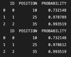
Afterwards, we print the change point table:
print(cp_part1_with_prune.collect())

print(cp_part1_without_prune.collect())
and we will see the output like this:
which shows that the results are the same under both settings regarding parameter 'prune'.
Further, we are to use the pruned model to detect the second part:
model_with_prune, cp_part2 = obcpd_with_prune.fit_predict(data=conn.table("PAL_ONLINE_BCPD_MOCK_TBL_PART2"), model=model_with_prune)

print(cp_part2.collect())
The results should be like this:
Finally, we plot all the change points in the original graph by orange vertical lines:

It's done! All the change points in two continuous segements have be detected.
Use Case II: Real World Sensor Data
In this example, we have a real-world sensor dataset with a length of 1500 and it is stored in a dataframe named df_sensor:

We divide it equally into 15 segments, each containing 100 data points. Then, we use the OnlineBCPD algorithm to continuously detect change points within the dataset using the following code snippet:
def createTableFromDataFrame(df, table_name, cc):

    dropTable(table_name, cc)

    dt_ml = dataframe.create_dataframe_from_pandas(cc, df, table_name = table_name)

    return dt_ml


obcpd = OnlineBCPD(threshold=0.5, prune=True)

figure(num=None, figsize=(16, 4), dpi=80, facecolor='w', edgecolor='k')

plt.plot(data)

for i in range(15):

    createTableFromDataFrame(df_sensor[i * 100 : (i + 1) * 100], "PAL_ONLINE_BCPD_SENSOR_DATA_TBL", conn)

    model_with_prune, cp = obcpd_with_prune.fit_predict(data=conn.table("PAL_ONLINE_BCPD_SENSOR_DATA_TBL"))

    for pos in cp.collect()["POSITION"]:

        plt.axvline(x=pos, color='orange', linestyle='dashed')
Finally, we will get the following graph:

Discussion and Summary
In this blog post, we introduced a novel SAP HANA ML algorithm designed for continuous change point detection in time series data, using the Python machine learning client for SAP HANA (hana-ml). Through multiple examples, we demonstrated the effectiveness of its detection capabilities and the memory-saving benefits achieved by using the 'prune' parameter.
If you want to learn more about hana-ml and SAP HANA Predictive Analysis Library (PAL), please refer to the following links:
Bayesian Change Point Dectection under Complex Time Series in Python Machine Learning Client for SAP...
Weibull Analysis using Python machine learning client for SAP HANA
Outlier Detection using Statistical Tests in Python Machine Learning Client for SAP HANA
Outlier Detection by Clustering using Python Machine Learning Client for SAP HANA
Outlier Detection with One-class Classification using Python Machine Learning Client for SAP HANA
Learning from Labeled Anomalies for Efficient Anomaly Detection using Python Machine Learning Client...
Additive Model Time-series Analysis using Python Machine Learning Client for SAP HANA
Import multiple excel files into a single SAP HANA table
COPD study, explanation and interpretability with Python machine learning client for SAP HANA
- SAP Managed Tags:
- Machine Learning
You must be a registered user to add a comment. If you've already registered, sign in. Otherwise, register and sign in.
Labels in this area
-
Agents
3 -
AI
5 -
AI Launchpad
2 -
Artificial Intelligence
2 -
Artificial Intelligence (AI)
3 -
Brainstorming
1 -
BTP
1 -
Business AI
2 -
Business Trends
1 -
Cloud Foundry
1 -
Data and Analytics (DA)
1 -
Design and Engineering
1 -
forecasting
1 -
GenAI
1 -
Generative AI
4 -
Generative AI Hub
4 -
Graph
1 -
Language Models
1 -
LlamaIndex
1 -
LLM
2 -
LLMs
2 -
Machine Learning
1 -
Machine learning using SAP HANA
1 -
Mistral AI
1 -
NLP (Natural Language Processing)
1 -
open source
1 -
OpenAI
1 -
Python
2 -
RAG
2 -
Retrieval Augmented Generation
1 -
SAP Build Process Automation
1 -
SAP HANA
1 -
SAP HANA Cloud
1 -
User Experience
1 -
user interface
1 -
Vector Database
3 -
Vector DB
1 -
Vector Similarity
1
Top kudoed authors
| User | Count |
|---|---|
| 4 | |
| 4 | |
| 3 | |
| 2 | |
| 2 | |
| 1 | |
| 1 |