
- SAP Community
- Products and Technology
- Supply Chain Management
- SCM Blogs by Members
- Statistical Forecasting in IBP- Manage Forecast Mo...
Supply Chain Management Blogs by Members
Learn about SAP SCM software from firsthand experiences of community members. Share your own post and join the conversation about supply chain management.
Turn on suggestions
Auto-suggest helps you quickly narrow down your search results by suggesting possible matches as you type.
Showing results for
kunalroy
Participant
Options
- Subscribe to RSS Feed
- Mark as New
- Mark as Read
- Bookmark
- Subscribe
- Printer Friendly Page
- Report Inappropriate Content
11-14-2022
2:59 PM
Introduction:
While the overall process of statistical forecasting is not that complicated (unless you get into advanced statistical models), there are some minor details in the “Manage Forecast Models” app which can be confusing. Here I am sharing a simple example to demonstrate the key technical features of the app for ease of understanding.
Example:
For this example, one Product-Location-Customer combination has been considered. While this might not be the most ideal level for forecasting in majority of cases, some businesses might still like to forecast at this detailed granularity. The level of forecasting does not matter in context of this blog.
Refer Fig. 01. “Actuals Qty.” is the key figure that stores sales history data. Just by looking at the data, you can notice a few things- values are missing for “MAY 2022” & “AUG 2022”. You may also notice that the value “1000” in “MAR 2022” is much higher compared to rest of the data set and is most likely an ‘outlier’. We will validate this assumption in the later sections.
“Manage Forecast Models” App has multiple tabs- GENERAL, PREPROCESSING STEPS, FORECASTING STEPS, POSTPROCESSING STEPS. Let us look at the individual settings sequentially.
GENERAL: The General Tab settings are shown in Fig. 02.
PREPROCESSING STEPS:
Next is the “PREPROCESSING STEPS” tab. This is where we add settings to correct sales history data for “Missing values” & “Outliers.” Multiple preprocessing steps can be added one after another in this tab. It is important to judge the sequence in which you want to run preprocessing steps because wrong sequence might lead to undesirable results. For example, let us say you want to “Substitute missing values” in the historical data using “Mean”(Fig. 03).
So, the “average(mean)” of the entire historical data set will be calculated, and the missing values are substituted by that “average.” While calculating the average, ‘1000’ which is most probably an outlier, also gets included in the calculation which might not be desirable.
Average= Sum of data points/No. of data points= 1595/10= 159.5 (note that the ‘null values’ are not included as valid data points while calculating ‘mean’. So, the denominator in this case is ‘10’ and not ‘12’). See excel output below (Fig. 04)
The example shown above was just to highlight the impact of a probable outlier on the calculation of substituting missing values. However, to proceed further, we will replace missing values by a ‘Given Value’, = 80 (Settings shown in Fig. 05).
After running statistical forecasting operator, the given value of ‘80’ gets substituted in place of missing values (Fig. 06).
After “Missing Values” are substituted, the next step is to check for “Outliers” and to correct them (note that there is no SAP recommended set of steps for preprocessing tasks. It depends on individual business needs. In some cases, users might want to run all combination of sequences of preprocessing tasks before deciding on the final approach).
In this case, we are going ahead with “Interquartile Range test” for “Outlier Detection.” See settings below (Fig. 07).
As “Substitute Missing Values” is the predecessor step for outlier detection and the Input key figure is same in both (Actuals Qty.), the output of that step automatically becomes the input for outlier detection step.
Fig. 08 shows how IQR(Inter Quartile Range), Lower & Upper bounds are calculated. The only “Actuals Qty.” value which is outside of the boundaries (<3.5 or >139.5) is ‘1000’ and hence it is detected as an outlier.
Since, the outlier correction method chosen by us is “Correction with tolerance excluding outliers,” tolerance(bounds) are now recalculated for the dataset excluding outlier(s).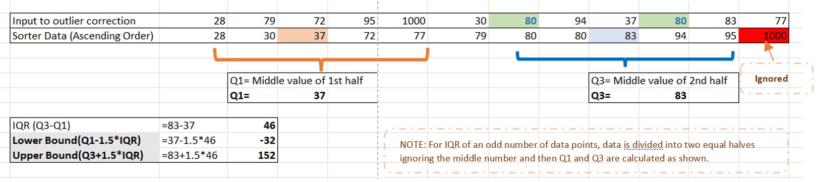
After running statistical forecasting, the upper bound value of ‘152’ (which is closer to 1000 than the lower bound value of -32) substitutes the value of ‘1000’.
FORECASTING STEPS:
This is where we define input & output key figures for forecasting and choose the forecasting algorithm.
It is important to note that even within the same forecasting model, the preprocessing steps might not always have direct connection to the forecasting step. It is only the input key figures for both these steps that can establish that connection.
For example, in Fig. 11, the main input for forecasting step is “Actuals Qty. Adj.” Now, this key figure has some manually adjusted values as shown in Fig. 12.
In the preprocessing steps for “substituting missing values” and “detecting & correcting outliers”, “Actuals Qty.” is taken as the input key figure while for forecasting step, a different key figure is now considered as input. So, forecasting output will have nothing to do with either “Actuals Qty.” key figure values or the output of the preprocessor steps.
Based on the settings in Fig. 11. Look at the Statistical Forecasting output(Fig. 13)using the simple average method. The forecasting output is a simple average of “Actuals Qty. Adj.” key figure:
You see that everything that we did as part of the Preprocessing step has not been considered as in input to Forecasting since a different key figure was chosen as main input for forecasting.
Now, let us consider the same key figure “Actuals Qty.” as the input to forecasting step as well (Fig. 14).
The actual input to statistical forecasting now is the final value of “Actuals Qty.” (corrected for both missing values & outliers). You can validate that by comparing the key figures “Stat Output for Outlier Correction” & “Target Key Figure for Calculated Forecast Input.” Both have the same values.
POSTPROCESSING STEPS:
In this step, we choose the error measure for comparison between Sales History & Ex-post forecast. In this example, MAPE has been chosen as the error measure (Fig. 16).
The standard MAPE key figure doesn’t have a time dimension associated with it. So, a custom key figure has to be created to make it time dependent (so it can be seen in excel planning view). There are several ways of doing it. For this example, I have used the following calculation (Fig. 16). MAPE results can be seen in Fig. 15 & Fig. 17.
I hope the example shared above simplifies the understanding around “Manage Forecast Models” app. I have tried to cover how the different tabs within the app link to each other and how output of one, influences other. You can read other posts relevant to IBP Demand at these links:
SAP Integrated Business Planning for demand | SAP | SAP Blogs
All Questions in SAP Integrated Business Planning for demand | SAP Community
Please feel free to share your feedback/thoughts.
While the overall process of statistical forecasting is not that complicated (unless you get into advanced statistical models), there are some minor details in the “Manage Forecast Models” app which can be confusing. Here I am sharing a simple example to demonstrate the key technical features of the app for ease of understanding.
Example:
For this example, one Product-Location-Customer combination has been considered. While this might not be the most ideal level for forecasting in majority of cases, some businesses might still like to forecast at this detailed granularity. The level of forecasting does not matter in context of this blog.
Refer Fig. 01. “Actuals Qty.” is the key figure that stores sales history data. Just by looking at the data, you can notice a few things- values are missing for “MAY 2022” & “AUG 2022”. You may also notice that the value “1000” in “MAR 2022” is much higher compared to rest of the data set and is most likely an ‘outlier’. We will validate this assumption in the later sections.

Fig. 01- “Actuals Qty.”- key figure to store sales history data.
“Manage Forecast Models” App has multiple tabs- GENERAL, PREPROCESSING STEPS, FORECASTING STEPS, POSTPROCESSING STEPS. Let us look at the individual settings sequentially.
GENERAL: The General Tab settings are shown in Fig. 02.
Fig.02- “GENERAL” tab settings.
PREPROCESSING STEPS:
Next is the “PREPROCESSING STEPS” tab. This is where we add settings to correct sales history data for “Missing values” & “Outliers.” Multiple preprocessing steps can be added one after another in this tab. It is important to judge the sequence in which you want to run preprocessing steps because wrong sequence might lead to undesirable results. For example, let us say you want to “Substitute missing values” in the historical data using “Mean”(Fig. 03).

Fig.03- PREPROCESSING STEPS- Method used for substitution- Mean
So, the “average(mean)” of the entire historical data set will be calculated, and the missing values are substituted by that “average.” While calculating the average, ‘1000’ which is most probably an outlier, also gets included in the calculation which might not be desirable.
Average= Sum of data points/No. of data points= 1595/10= 159.5 (note that the ‘null values’ are not included as valid data points while calculating ‘mean’. So, the denominator in this case is ‘10’ and not ‘12’). See excel output below (Fig. 04)

Fig.04- After running the ‘statistical forecasting’ operator, 159.5 is substituted in MAY and AUG where values were missing earlier.
The example shown above was just to highlight the impact of a probable outlier on the calculation of substituting missing values. However, to proceed further, we will replace missing values by a ‘Given Value’, = 80 (Settings shown in Fig. 05).
Fig. 05- PREPROCESSING STEPS- Method used for substitution- Given Value of 80.
After running statistical forecasting operator, the given value of ‘80’ gets substituted in place of missing values (Fig. 06).

Fig. 06- After running ‘statistical forecasting’ operator, ‘80’ is substituted in MAY and AUG.
After “Missing Values” are substituted, the next step is to check for “Outliers” and to correct them (note that there is no SAP recommended set of steps for preprocessing tasks. It depends on individual business needs. In some cases, users might want to run all combination of sequences of preprocessing tasks before deciding on the final approach).
In this case, we are going ahead with “Interquartile Range test” for “Outlier Detection.” See settings below (Fig. 07).
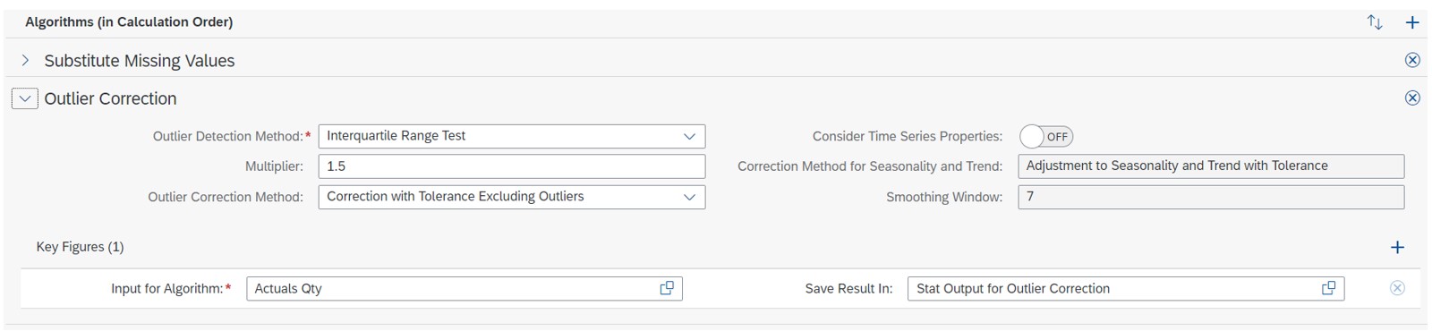
Fig. 07- PREPROCESSING STEPS- Settings for Outlier detection and correction
As “Substitute Missing Values” is the predecessor step for outlier detection and the Input key figure is same in both (Actuals Qty.), the output of that step automatically becomes the input for outlier detection step.
Fig. 08- Outlier Detection- Calculation of IQR, LB and UB.
Fig. 08 shows how IQR(Inter Quartile Range), Lower & Upper bounds are calculated. The only “Actuals Qty.” value which is outside of the boundaries (<3.5 or >139.5) is ‘1000’ and hence it is detected as an outlier.
Since, the outlier correction method chosen by us is “Correction with tolerance excluding outliers,” tolerance(bounds) are now recalculated for the dataset excluding outlier(s).
Fig. 09- Outlier Correction- Calculation of new boundaries(tolerances) for substituting outliers.
After running statistical forecasting, the upper bound value of ‘152’ (which is closer to 1000 than the lower bound value of -32) substitutes the value of ‘1000’.
Fig.10- After running ‘statistical forecasting’ operator, 152 is substituted for 1000 in MAR.
FORECASTING STEPS:
This is where we define input & output key figures for forecasting and choose the forecasting algorithm.
It is important to note that even within the same forecasting model, the preprocessing steps might not always have direct connection to the forecasting step. It is only the input key figures for both these steps that can establish that connection.
For example, in Fig. 11, the main input for forecasting step is “Actuals Qty. Adj.” Now, this key figure has some manually adjusted values as shown in Fig. 12.

Fig. 11- FORECASTING STEPS- Settings with “Actuals Qty. Adj.” as input key figure.

Fig.12- Actuals Qty. Adj. Key figure values highlighted above.
In the preprocessing steps for “substituting missing values” and “detecting & correcting outliers”, “Actuals Qty.” is taken as the input key figure while for forecasting step, a different key figure is now considered as input. So, forecasting output will have nothing to do with either “Actuals Qty.” key figure values or the output of the preprocessor steps.
Based on the settings in Fig. 11. Look at the Statistical Forecasting output(Fig. 13)using the simple average method. The forecasting output is a simple average of “Actuals Qty. Adj.” key figure:

Fig. 13- After running the ‘statistical forecasting’ operator, Statistical Forecast is generated based on “Actuals Qty. Adj.”.
You see that everything that we did as part of the Preprocessing step has not been considered as in input to Forecasting since a different key figure was chosen as main input for forecasting.
Now, let us consider the same key figure “Actuals Qty.” as the input to forecasting step as well (Fig. 14).

Fig. 14- FORECASTING STEPS- Settings with “Actuals Qty.” as input key figure.
The actual input to statistical forecasting now is the final value of “Actuals Qty.” (corrected for both missing values & outliers). You can validate that by comparing the key figures “Stat Output for Outlier Correction” & “Target Key Figure for Calculated Forecast Input.” Both have the same values.

Fig. 15- After running ‘statistical forecasting’ operator, Statistical Forecast is generated based on “Actuals Qty.” corrected for missing values and outliers.
POSTPROCESSING STEPS:
In this step, we choose the error measure for comparison between Sales History & Ex-post forecast. In this example, MAPE has been chosen as the error measure (Fig. 16).

Fig. 16- POSTPROCESSING STEPS- MAPE selected as target error measure.
The standard MAPE key figure doesn’t have a time dimension associated with it. So, a custom key figure has to be created to make it time dependent (so it can be seen in excel planning view). There are several ways of doing it. For this example, I have used the following calculation (Fig. 16). MAPE results can be seen in Fig. 15 & Fig. 17.

Fig. 17- After Statistical Forecasting Operator Run, MAPE is calculated as 45.632%.

Fig. 18- Custom Key figure to show MAPE values in Excel.
I hope the example shared above simplifies the understanding around “Manage Forecast Models” app. I have tried to cover how the different tabs within the app link to each other and how output of one, influences other. You can read other posts relevant to IBP Demand at these links:
SAP Integrated Business Planning for demand | SAP | SAP Blogs
All Questions in SAP Integrated Business Planning for demand | SAP Community
Please feel free to share your feedback/thoughts.
1 Comment
You must be a registered user to add a comment. If you've already registered, sign in. Otherwise, register and sign in.
Labels in this area
-
aATP
1 -
ABAP Programming
1 -
Activate Credit Management Basic Steps
1 -
Adverse media monitoring
1 -
Alerts
1 -
Ausnahmehandling
1 -
bank statements
1 -
Bin Sorting sequence deletion
1 -
Bin Sorting upload
1 -
BP NUMBER RANGE
1 -
Brazil
1 -
Business partner creation failed for organizational unit
1 -
Business Technology Platform
1 -
Central Purchasing
1 -
Charge Calculation
2 -
Cloud Extensibility
1 -
Compliance
1 -
Controlling
1 -
Controlling Area
1 -
Data Enrichment
1 -
DIGITAL MANUFACTURING
1 -
digital transformation
1 -
Dimensional Weight
1 -
Direct Outbound Delivery
1 -
E-Mail
1 -
ETA
1 -
EWM
6 -
EWM - Delivery Processing
2 -
EWM - Goods Movement
3 -
EWM Outbound configuration
1 -
EWM-RF
1 -
EWM-TM-Integration
1 -
Extended Warehouse Management (EWM)
3 -
Extended Warehouse Management(EWM)
7 -
Finance
1 -
Freight Settlement
1 -
Geo-coordinates
1 -
Geo-routing
1 -
Geocoding
1 -
Geographic Information System
1 -
GIS
1 -
Goods Issue
2 -
GTT
2 -
IBP inventory optimization
1 -
inbound delivery printing
1 -
Incoterm
1 -
Innovation
1 -
Inspection lot
1 -
intraday
1 -
Introduction
1 -
Inventory Management
1 -
Localization
1 -
Logistics Optimization
1 -
Map Integration
1 -
Material Management
1 -
Materials Management
1 -
MFS
1 -
Outbound with LOSC and POSC
1 -
Packaging
1 -
PPF
1 -
PPOCE
1 -
PPOME
1 -
print profile
1 -
Process Controllers
1 -
Production process
1 -
QM
1 -
QM in procurement
1 -
Real-time Geopositioning
1 -
Risk management
1 -
S4 HANA
1 -
S4-FSCM-Custom Credit Check Rule and Custom Credit Check Step
1 -
S4SCSD
1 -
Sales and Distribution
1 -
SAP DMC
1 -
SAP ERP
1 -
SAP Extended Warehouse Management
2 -
SAP Hana Spatial Services
1 -
SAP IBP IO
1 -
SAP MM
1 -
sap production planning
1 -
SAP QM
1 -
SAP REM
1 -
SAP repetiative
1 -
SAP S4HANA
1 -
SAP Transportation Management
2 -
SAP Variant configuration (LO-VC)
1 -
SD (Sales and Distribution)
1 -
Source inspection
1 -
Storage bin Capacity
1 -
Supply Chain
1 -
Supply Chain Disruption
1 -
Supply Chain for Secondary Distribution
1 -
Technology Updates
1 -
TMS
1 -
Transportation Cockpit
1 -
Transportation Management
2 -
Visibility
2 -
warehouse door
1 -
WOCR
1
Related Content
- SAP Intelligent Clinical Supply Management goes CTS Europe 2024 – our key insights in Supply Chain Management Blogs by SAP
- “Mind the Gap” – Improves ROI, Cost & Margin by Merging Planning Processes in Supply Chain Management Blogs by SAP
- Transfer Purchase Requisitions as FORECAST from S4 to IBP Time Series Planning Area Key Figure in Supply Chain Management Q&A
- Attach Rate Planning in IBP in Supply Chain Management Blogs by Members
- statistical forecast key figure dissag issue for sales org level in Supply Chain Management Q&A
Top kudoed authors
| User | Count |
|---|---|
| 3 | |
| 2 | |
| 2 | |
| 2 | |
| 1 | |
| 1 | |
| 1 | |
| 1 | |
| 1 | |
| 1 |