
- SAP Community
- Products and Technology
- Technology
- Technology Blogs by SAP
- Build historization and track data changes with SA...
Technology Blogs by SAP
Learn how to extend and personalize SAP applications. Follow the SAP technology blog for insights into SAP BTP, ABAP, SAP Analytics Cloud, SAP HANA, and more.
Turn on suggestions
Auto-suggest helps you quickly narrow down your search results by suggesting possible matches as you type.
Showing results for
Product and Topic Expert
Options
- Subscribe to RSS Feed
- Mark as New
- Mark as Read
- Bookmark
- Subscribe
- Printer Friendly Page
- Report Inappropriate Content
11-10-2022
8:33 AM
Overview
When visualizing and working with data over a time perspective there are at least 3 scenarios:
- non-temporal: We only want to analyze the latest data available. This is the default approach when building presentations. It gives us the opportunity to quickly model data and build reports on top of it.
- temporal (no monitoring): We want to analyze data over a specific timeline. This is needed for building time series charts and gaining insights from the past
- temporal (data changes monitoring): We want to analyze data over a specific timeframe. Additionally, we want to know when the underlying data has changed and also have an overview of all changes.

This blog includes basic ways to implement historization in SAP Data Warehouse Cloud (DWC) and track data changes inside the Data Builder. This is only one way of doing it. There might be better/other ways and also especially for scenario 3 there might be upcoming features in the future that help us with tracking data changes.
This blog does not include slowly changing dimensions.
Implementation
Scenario 1 (non temporal)
We can use standard DWC functionality for data integration. Both Remote Tables and Data Flows can be scheduled to provide the current data from the underlying source.
Data Flows can be scheduled hourly as the smallest interval and also be manually triggered.
Remote Tables can be scheduled and manually triggered just as Data Flows and also be configured to replicate data in real time. For real-time replication, some additional prerequisites have to be met.
Scenario 2 (temporal, no monitoring)
We can use Data Flows to build historization. With scheduled Data Flows, we can build a history of data of different granularity, hourly being the smallest.
Inside the Data Flow, everything we have to do is to insert a timestamp. We do this by adding a projection between the source and the target and creating a calculated column inside the projection. We use the function "Current_Date()", which is sufficient as a "timestamp" for us. For more accuracy, the function "Current_Timestamp()" can be used. There are more date functions supported.
Below you see the Data Flow as well as the data preview after performing four data loads.

Data Flow with timestamp
Now as time progresses, our data will build up and more and more insights will be gained from any time-based analysis. Please keep in mind that the smaller the increment of the historization the larger the amount of data stored in DWC. 100.000 records loaded on a weekly basis might be 16.800.000 if loaded hourly.
In some cases there might be a data history available in the source system. This can be loaded into DWC all at once and extended by our daily/weekly/etc. loads.
Scenario 3 (temporal, data changes monitoring)
We can now use basic data modeling to gain insights about data changes. We will know IF our data has changed compared with the past and also WHAT and HOW it changed.
For this scenario we use the historization we built in Scenario 2.
In our usecase we would like to compare the data to the data loaded one day earlier. For this, we build a new view. It is based on our TR_productHistory table (target of the Data Flow in step 2) joined by itself. For this join, one of the tables represents the data as of today and one table represents the data as of yesterday. To build this logic, we need an additional column in our "today" table, which will enable us to join it with the "yesterday" table.
ADD_DAYS("Date of Dataload", -1)Its important to understand the logic of this column: Here we calculate the date to which we want to compare our data. So if you want to see how the data changed from yesterday to today, use the function above. If you would like to compare the data to how it was a week ago the function would be "ADD_DAYS("Date of DataLoad", -7)". Most times, this is in line with the dataload frequency you chose in Scenario 2.
Now, choose the correct join columns as seen below.
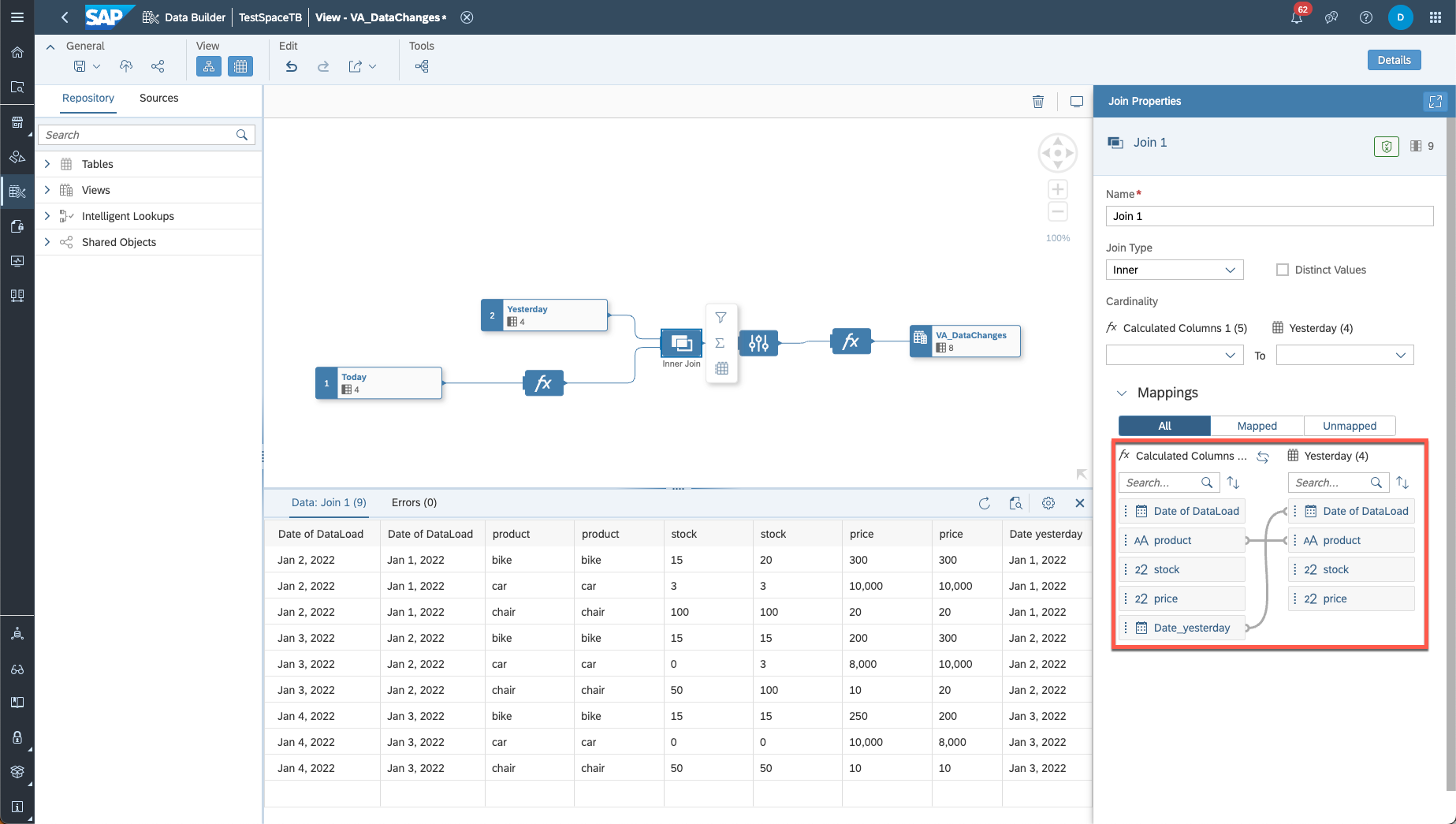
join operator
In the projection, multiple columns will be removed because the names are not distinct. Make sure to restore the columns for which you want to see the data changes. Also rename the column from "yesterday" accordingly.
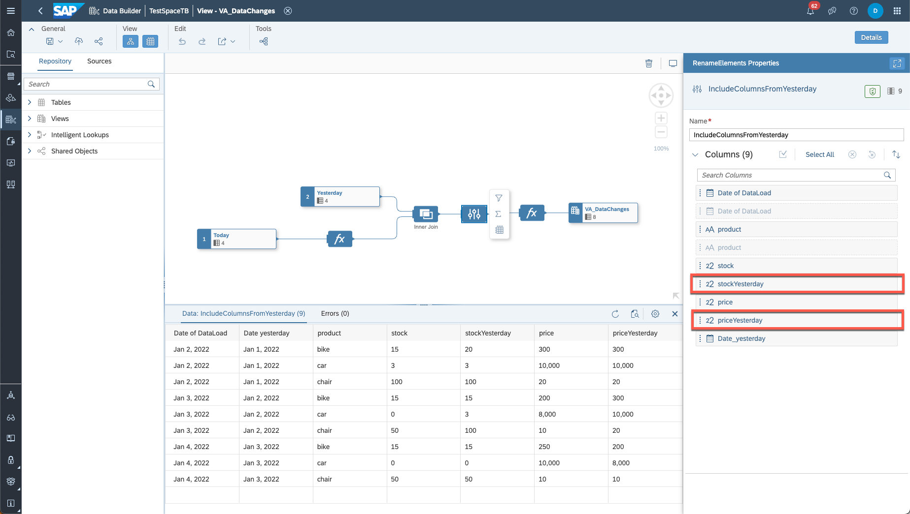
Restore columns for data change tracking
Now we have a data preview where we already see data changes. Keep in mind that the first day of our data loading is not represented here because for this day we don't have any data for "yesterday". If you nevertheless keep the data for the first day, perform a left (or right) join instead of inner join.
With this data preparation we are now able to include calculated columns where we track the changes. There are multiple possibilities depending on what you want to track. Here are a few examples:
Did the price change since yesterday?
This calculation will display the date of the dataload if the price of the product changed that day.

Insert calculated column
How much did the stock change since yesterday?
This calculation will display the amount of the stock change (only possible for numbers)
stock - stockYesterdayDid anything change at all?
This calculation will give data change information over multiple columns (can be all columns)
case when stock != stockYersterday or price != priceYesterday then true else false endWe can change the calculation to whatever we need in our visualization. Also we can have multiple calculated columns for all kinds of data changes (for each column, for different analyses etc.).
Also, for scenario 3 we do not integrate any additional data into DWC. We just build a view on the dataloads from scenario 2. This gives us the option to add monitoring at any given point while still being able to track data changes for ALL our data.
Conclusion & Outlook
There are lots of ways to analyze and monitor historical data. There might be options we can utilize when working with specific data sources but this blog can be used for ALL data source that offer data flows.
I feel like lots of historization capabilites, that other DWH tools might offer can be compensated by a stable data modeling approach. Also there might be great ways with python scripting too.
The future might bring additional functionalities to DWC for this topic. For now, feel free to use this approach and adjust it to your use case.
- SAP Managed Tags:
- SAP Analytics Cloud, data modeling,
- SAP Datasphere,
- Cloud
Labels:
You must be a registered user to add a comment. If you've already registered, sign in. Otherwise, register and sign in.
Labels in this area
-
ABAP CDS Views - CDC (Change Data Capture)
2 -
AI
1 -
Analyze Workload Data
1 -
BTP
1 -
Business and IT Integration
2 -
Business application stu
1 -
Business Technology Platform
1 -
Business Trends
1,658 -
Business Trends
93 -
CAP
1 -
cf
1 -
Cloud Foundry
1 -
Confluent
1 -
Customer COE Basics and Fundamentals
1 -
Customer COE Latest and Greatest
3 -
Customer Data Browser app
1 -
Data Analysis Tool
1 -
data migration
1 -
data transfer
1 -
Datasphere
2 -
Event Information
1,400 -
Event Information
66 -
Expert
1 -
Expert Insights
177 -
Expert Insights
299 -
General
1 -
Google cloud
1 -
Google Next'24
1 -
Kafka
1 -
Life at SAP
780 -
Life at SAP
13 -
Migrate your Data App
1 -
MTA
1 -
Network Performance Analysis
1 -
NodeJS
1 -
PDF
1 -
POC
1 -
Product Updates
4,577 -
Product Updates
345 -
Replication Flow
1 -
RisewithSAP
1 -
SAP BTP
1 -
SAP BTP Cloud Foundry
1 -
SAP Cloud ALM
1 -
SAP Cloud Application Programming Model
1 -
SAP Datasphere
2 -
SAP S4HANA Cloud
1 -
SAP S4HANA Migration Cockpit
1 -
Technology Updates
6,873 -
Technology Updates
427 -
Workload Fluctuations
1
Related Content
- 体验更丝滑!SAP 分析云 2024.07 版功能更新 in Technology Blogs by SAP
- What’s New in SAP Analytics Cloud Release 2024.08 in Technology Blogs by SAP
- ad-hoc analysis on BW Querys in SAP Analytics Cloud on iOS mobile devices in Technology Q&A
- SAP Query / ABAP in Technology Q&A
- Inventory Warehouse Report in Technology Q&A
Top kudoed authors
| User | Count |
|---|---|
| 40 | |
| 25 | |
| 17 | |
| 14 | |
| 8 | |
| 7 | |
| 7 | |
| 7 | |
| 6 | |
| 6 |