
- SAP Community
- Products and Technology
- Technology
- Technology Blogs by SAP
- Value Driver Tree (VDT) Update – Deprecation of Le...
Technology Blogs by SAP
Learn how to extend and personalize SAP applications. Follow the SAP technology blog for insights into SAP BTP, ABAP, SAP Analytics Cloud, SAP HANA, and more.
Turn on suggestions
Auto-suggest helps you quickly narrow down your search results by suggesting possible matches as you type.
Showing results for
Advisor
Options
- Subscribe to RSS Feed
- Mark as New
- Mark as Read
- Bookmark
- Subscribe
- Printer Friendly Page
- Report Inappropriate Content
11-02-2022
9:51 AM
The legacy VDT will be, after co-existing with the new VDT in stories for some time, deprecated in SAP Analytics Cloud.
The planned deprecation timeline will be as follow:
Legacy VDT:
Of course, this does not mean that legacy VDTs should be discarded – a manual migration into the new VDT in stories is still possible before the deprecation in story and boardroom in QRC2 2023. Generally, the migration method consists of first bringing the legacy VDT into a classic story (as VDT widget) and the subsequent adjustments of specific calculations there.
(Note: After the migration, do not convert the classic story into optimized view mode just yet, to continue copy/pasting the migrated VDT into further artefacts. It is planned to also enable this ability for stories in optimized view mode for future releases.)
In this blog post we’re going through the migration of a sample VDT together. So let’s get started!
We’re starting out with this legacy VDT:
We shall now transform it into a new VDT widget that looks and behaves exactly like the original but enables us to benefit from latest innovations in SAP Analytics Cloud, such as the new model and optimized design experience.
The initial migration step will already trigger automatic migration for all nodes possible. This initial step is carried out by bringing a VDT widget into a classic story, selecting Display Existing Value Driver Tree, opening the builder panel and triggering the Transform button. The result already looks familiar, but you will spot differences, which we will tackle manually in the following steps.
One of the main differences between new and legacy VDT is that the new VDT doesn’t allow to explicitly trigger a simulation like it was done before. Instead, all calculations are performed instantly after data has changed. We’ll use model calculations and story calculations to achieve this. In our example we will set our new VDT widget to show a version without the data that was previously written by legacy VDT simulation, so it’s easier to spot the gaps requiring calculation input/adjustments. With the simulation data removed, our VDT looks like this:
You will notice that all nodes have been converted to data source nodes. All nodes that have already been data source nodes before should work as expected and do not require manual rework.
So, now let’s tackle the gaps one by one. We’ll start with the volume node. It was a year-over-year node in the legacy VDT. We will now create the year-over-year calculation with the new iterate formula in the model. So let’s head over to the modeler and add a new account volume_yoy. We add the iterate formula like shown in the screenshot below. The formula takes the value from the first year of the calculation from the Volume account and then grows it year over year by applying Market Share Growth as growth factor to the value of the previous year.
The formula above also utilizes the inverse function to enable the calculated account for data entry. If you enter data here – whether in a VDT or table widget – it will modify the Market Share Growth account then. When we set this new volume_yoy account on the volume node in our VDT, this gives us the data we want:
The expense node in this sample VDT can be treated in a similar fashion.
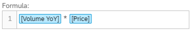
The revenue node in our VDT was previously a simple calculation node that calculated price times volume. We can simply mirror this calculation in the model by entering a matching formula. Note that you can create much more complex calculations here than was possible with simple calculation nodes in VDTs alone. Also note that if your legacy VDT node used to calculate on details instead of aggregate, you need to set up exception aggregation dimensions correctly for the account in the modeler as well. Very likely you did this already, so your sums show up correctly in grids. In this example case we set the product and date dimension as exception aggregation, so that the price*volume calculation for each product is done before the aggregation. See this help article for details on when and how to use exception aggregations if your calculations need to be performed on details.

Last one left is the Balance node. In our legacy VDT this was a union node that united the revenue and expense nodes. The best way to do this with new VDTs is to set up your accounts in a hierarchy, so they automatically sum up properly. Of course you could again use any calculation that sums up individual accounts. In our example, we introduce a new balance account and set it as the parent for the Revenue and Expenses accounts, so they sum up automatically.
Check out additional information on migration of legacy VDTs and the VDT widget:
A big thank you to André Seiffert for a great collaboration and providing most of the input to this blog post!
The planned deprecation timeline will be as follow:
Legacy VDT:
- 2022 QRC4:
- Can be opened, viewed, and executed in VDT designer
- Can no longer be created, copied, or edited, but will remain functional in stories and boardroom
- 2023 QRC2:
- Can be opened, viewed, and executed in VDT designer
- Can no longer be viewed in stories and boardroom (Replaced by placeholders)
- 2023 QRC3:
- Legacy VDT designer will be completely removed, meaning there will be no more access to legacy VDT
Of course, this does not mean that legacy VDTs should be discarded – a manual migration into the new VDT in stories is still possible before the deprecation in story and boardroom in QRC2 2023. Generally, the migration method consists of first bringing the legacy VDT into a classic story (as VDT widget) and the subsequent adjustments of specific calculations there.
(Note: After the migration, do not convert the classic story into optimized view mode just yet, to continue copy/pasting the migrated VDT into further artefacts. It is planned to also enable this ability for stories in optimized view mode for future releases.)
In this blog post we’re going through the migration of a sample VDT together. So let’s get started!
We’re starting out with this legacy VDT:

Example of legacy VDT before migration
We shall now transform it into a new VDT widget that looks and behaves exactly like the original but enables us to benefit from latest innovations in SAP Analytics Cloud, such as the new model and optimized design experience.
Partial Automatic Migration
The initial migration step will already trigger automatic migration for all nodes possible. This initial step is carried out by bringing a VDT widget into a classic story, selecting Display Existing Value Driver Tree, opening the builder panel and triggering the Transform button. The result already looks familiar, but you will spot differences, which we will tackle manually in the following steps.

Check your VDT after the partial automatic migration for nodes requiring adjustments
One of the main differences between new and legacy VDT is that the new VDT doesn’t allow to explicitly trigger a simulation like it was done before. Instead, all calculations are performed instantly after data has changed. We’ll use model calculations and story calculations to achieve this. In our example we will set our new VDT widget to show a version without the data that was previously written by legacy VDT simulation, so it’s easier to spot the gaps requiring calculation input/adjustments. With the simulation data removed, our VDT looks like this:

Remove simulation results to spot gaps requiring calculation input/adjustments
Data Source Nodes
You will notice that all nodes have been converted to data source nodes. All nodes that have already been data source nodes before should work as expected and do not require manual rework.
YoY Node
So, now let’s tackle the gaps one by one. We’ll start with the volume node. It was a year-over-year node in the legacy VDT. We will now create the year-over-year calculation with the new iterate formula in the model. So let’s head over to the modeler and add a new account volume_yoy. We add the iterate formula like shown in the screenshot below. The formula takes the value from the first year of the calculation from the Volume account and then grows it year over year by applying Market Share Growth as growth factor to the value of the previous year.

The iterate formula
The formula above also utilizes the inverse function to enable the calculated account for data entry. If you enter data here – whether in a VDT or table widget – it will modify the Market Share Growth account then. When we set this new volume_yoy account on the volume node in our VDT, this gives us the data we want:

Year over year calculation results
The expense node in this sample VDT can be treated in a similar fashion.
Simple Calculation Node
The revenue node in our VDT was previously a simple calculation node that calculated price times volume. We can simply mirror this calculation in the model by entering a matching formula. Note that you can create much more complex calculations here than was possible with simple calculation nodes in VDTs alone. Also note that if your legacy VDT node used to calculate on details instead of aggregate, you need to set up exception aggregation dimensions correctly for the account in the modeler as well. Very likely you did this already, so your sums show up correctly in grids. In this example case we set the product and date dimension as exception aggregation, so that the price*volume calculation for each product is done before the aggregation. See this help article for details on when and how to use exception aggregations if your calculations need to be performed on details.
The price*volume calculation is an example requiring exception aggregation
Union node
Last one left is the Balance node. In our legacy VDT this was a union node that united the revenue and expense nodes. The best way to do this with new VDTs is to set up your accounts in a hierarchy, so they automatically sum up properly. Of course you could again use any calculation that sums up individual accounts. In our example, we introduce a new balance account and set it as the parent for the Revenue and Expenses accounts, so they sum up automatically.


A way to unite two nodes is to create a new parent node for both
Check out additional information on migration of legacy VDTs and the VDT widget:
A big thank you to André Seiffert for a great collaboration and providing most of the input to this blog post!
- SAP Managed Tags:
- SAP Analytics Cloud,
- SAP Analytics Cloud for planning,
- Data and Analytics
Labels:
You must be a registered user to add a comment. If you've already registered, sign in. Otherwise, register and sign in.
Labels in this area
-
ABAP CDS Views - CDC (Change Data Capture)
2 -
AI
1 -
Analyze Workload Data
1 -
BTP
1 -
Business and IT Integration
2 -
Business application stu
1 -
Business Technology Platform
1 -
Business Trends
1,658 -
Business Trends
91 -
CAP
1 -
cf
1 -
Cloud Foundry
1 -
Confluent
1 -
Customer COE Basics and Fundamentals
1 -
Customer COE Latest and Greatest
3 -
Customer Data Browser app
1 -
Data Analysis Tool
1 -
data migration
1 -
data transfer
1 -
Datasphere
2 -
Event Information
1,400 -
Event Information
66 -
Expert
1 -
Expert Insights
177 -
Expert Insights
293 -
General
1 -
Google cloud
1 -
Google Next'24
1 -
Kafka
1 -
Life at SAP
780 -
Life at SAP
13 -
Migrate your Data App
1 -
MTA
1 -
Network Performance Analysis
1 -
NodeJS
1 -
PDF
1 -
POC
1 -
Product Updates
4,577 -
Product Updates
340 -
Replication Flow
1 -
RisewithSAP
1 -
SAP BTP
1 -
SAP BTP Cloud Foundry
1 -
SAP Cloud ALM
1 -
SAP Cloud Application Programming Model
1 -
SAP Datasphere
2 -
SAP S4HANA Cloud
1 -
SAP S4HANA Migration Cockpit
1 -
Technology Updates
6,873 -
Technology Updates
419 -
Workload Fluctuations
1
Related Content
- Identity Provisioning Documentation Joined the Family of SAP Cloud Identity Services in Technology Blogs by SAP
- What’s New in SAP HANA Cloud – March 2024 in Technology Blogs by SAP
- What's New in the Newly Repackaged SAP Integration Suite, advanced event mesh in Technology Blogs by SAP
- How SAP’s Generative AI Hub facilitates embedded, trustworthy, and reliable AI in Technology Blogs by SAP
- How to load customers (business partners) in S/4 HANA with Winshuttle in Technology Blogs by Members
Top kudoed authors
| User | Count |
|---|---|
| 35 | |
| 25 | |
| 13 | |
| 7 | |
| 7 | |
| 6 | |
| 6 | |
| 6 | |
| 5 | |
| 4 |