
- SAP Community
- Products and Technology
- Technology
- Technology Blogs by SAP
- Python hana_ml: Basic Auto ML Classification(Autom...
Technology Blogs by SAP
Learn how to extend and personalize SAP applications. Follow the SAP technology blog for insights into SAP BTP, ABAP, SAP Analytics Cloud, SAP HANA, and more.
Turn on suggestions
Auto-suggest helps you quickly narrow down your search results by suggesting possible matches as you type.
Showing results for
Advisor
Options
- Subscribe to RSS Feed
- Mark as New
- Mark as Read
- Bookmark
- Subscribe
- Printer Friendly Page
- Report Inappropriate Content
09-21-2022
7:58 AM
I am writing this blog to show basic Auto ML classification training procedures using python package hana_ml. Wtih class AutomaticClassification, you don't need to consider the both preprocessing and classification algorithms. AutoML finds the best one.
Environment
Environment is as below.
- Python: 3.7.3(Not Google Colaboratory)
- HANA: Cloud Edition 2022.16
Python packages and their versions.
- hana_ml: 2.14.22091801
- pandas: 1.3.0
- scikit-learn: 1.0.2
As for HANA Cloud, I activated scriptserver and created my users. Though I don't recognize other special configurations, I may miss something since our HANA Cloud was created long time before.
I didn't use HDI here to make environment simple.
Best Pipeline Report
Firstly let me show you a best pipeline report. The report can be displayed within jupyter or downloaded as html file.
Overview
It consists of upper and lower blocks. Pipeline list is displayed on the upper part. Metrics, Pipelines and Logs are displayed on the lower block.

Metrics
In "Metrics" tab, there are the below metrics. I trained with default target scoring, so all metrics are AUC related. It depends on parameter "scorings".
- AUC-ID
- ACCURACY-AUC
- F1_SCORE_0-AUC / F1_SCORE_1-AUC
- KAPPA-AUC
- LAYERS-AUC
- MCC-AUC
- PRECISION_0-AUC / PRECISION_1-AUC
- RECALL_0-AUC / RECALL_1-AUC
- SUPPORT_0-AUC / SUPPORT_1-AUC


Pipelines
Pipelines tab screen shows the best pipelines.

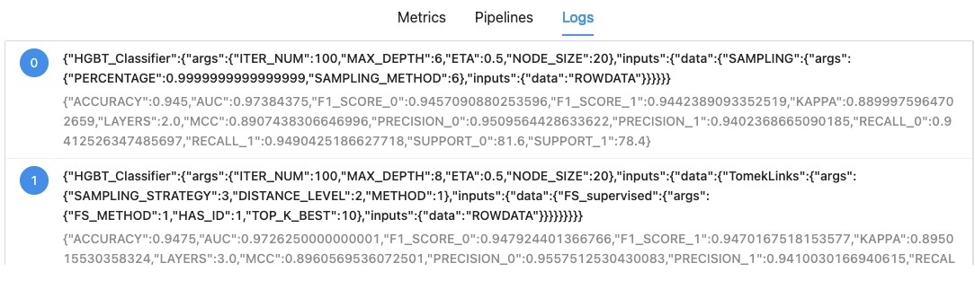
Logs
There are logs of the pipelines.
Pipeline Progress Status Monitor
Pipeline Progress Status Monitor shows Auto ML progress.
Generation Detail

Execution Logs

Python Script
1. Install Python packages
Install python package hana_ml and scikit-learn.
!pip install hana_ml scikit-learn2. Import modules
Import python package modules.
import json

import pprint

import uuid


from hana_ml.algorithms.pal.partition import train_test_val_split

from hana_ml.algorithms.pal.auto_ml import AutomaticClassification

from hana_ml.dataframe import ConnectionContext, create_dataframe_from_pandas

from hana_ml.model_storage import ModelStorage

from hana_ml.visualizers.automl_progress import PipelineProgressStatusMonitor

from hana_ml.visualizers.automl_report import BestPipelineReport

import pandas as pd

from sklearn.datasets import make_classification
3. Connect to HANA Cloud
Connect to HANA Cloud and check its version.
ConnectionContext class is for connection to HANA.
HOST = '<HANA HOST NAME>'

SCHEMA = USER = '<USER NAME>'

PASS = '<PASSWORD>'

conn = ConnectionContext(address=HOST, port=443, user=USER,

                           password=PASS, schema=SCHEMA,

                           encrypt=True, sslValidateCertificate=False)

print(conn.hana_version())
4.00.000.00.1660640318 (fa/CE2022.16)4. Create test data
Create test data using scikit-learn.
There are 3 features and 1 target variable.
def make_df():

    X, y = make_classification(n_samples=1000,

                               n_features=3, n_redundant=0)

    df = pd.DataFrame(X, columns=['X1', 'X2', 'X3'])

    df['CLASS'] = y

    return df


df = make_df()

print(df)

df.info()
Here is dataframe overview.
           X1        X2        X3  CLASS

0    0.964229  1.995667  0.244143      1

1   -1.358062 -0.254956  0.502890      0

2    1.732057  0.261251 -2.214177      1

3   -1.519878  1.023710 -0.262691      0

4    4.020262  1.381454 -1.582143      1

..        ...       ...       ...    ...

995 -0.247950  0.500666 -0.219276      1

996 -1.918810  0.183850 -1.448264      0

997 -0.605083 -0.491902  1.889303      0

998 -0.742692  0.265878 -0.792163      0

999  2.189423  0.742682 -2.075825      1


[1000 rows x 4 columns]

<class 'pandas.core.frame.DataFrame'>

RangeIndex: 1000 entries, 0 to 999

Data columns (total 4 columns):

 #   Column  Non-Null Count  Dtype

---  ------  --------------  -----

 0   X1      1000 non-null   float64

 1   X2      1000 non-null   float64

 2   X3      1000 non-null   float64

 3   CLASS   1000 non-null   int64

dtypes: float64(3), int64(1)

memory usage: 31.4 KB
5. define table and upload data
Define HANA Table and upload data using function "create_dataframe_from_pandas".
The function is very useful, since it automatically define table and upload at the same time. Please check options for further detail.
TRAIN_TABLE = 'PAL_TRAIN'

dfh = create_dataframe_from_pandas(conn, df, TRAIN_TABLE,

                             schema=SCHEMA,

                             force=True, # True: truncate and insert

                             replace=True) # True: Null is replaced by 0
6. Split data into train and test dataset
Split dataset using function "train_test_val_split". The function needs key columns, so I added key column using function "add_id".
train, test, _ = train_test_val_split(dfh.add_id(),

                                      testing_percentage=0.2,

                                      validation_percentage=0)

print(f'Train shape: {train.shape}, Test Shape: {test.shape}')
Train shape: [8000, 5], Test Shape: [2000, 5]7. Prepare for Training
Train by using class "AutomaticClassification". "progress_id" is a key to identify the classification job.
# AutomaticClassification init

progress_id = "automl_{}".format(uuid.uuid1())

auto_c = AutomaticClassification(progress_indicator_id=progress_id)
Here, you can use workload class to manage HANA workload.
Before executing training, you have to execute "CREATE WORKLOAD CLASS" SQL like below.
CREATE WORKLOAD CLASS "PAL_AUTOML_WORKLOAD" SET 'PRIORITY' = '3', 'STATEMENT MEMORY LIMIT' = '4' , 'STATEMENT THREAD LIMIT' = '20';Here is python script to use the workload class.
# enable_workload_class

auto_c.enable_workload_class(workload_class_name="PAL_AUTOML_WORKLOAD")
You can check called algorithms and their parameters.
>> auto_c.display_config_dict()

       Used Operators     Category

0              CATPCA  Transformer

1       FS_supervised  Transformer

2     FS_unsupervised  Transformer

3     HGBT_Classifier   Classifier

4      MLP_Classifier   Classifier

5   M_LOGR_Classifier   Classifier

6       NB_Classifier   Classifier

7      RDT_Classifier   Classifier

8      SVM_Classifier   Classifier

9       DT_Classifier   Classifier

10           SAMPLING    Resampler

11              SMOTE    Resampler

12         SMOTETomek    Resampler

13         TomekLinks    Resampler


------------------------------------------------------------


CATPCA

......


                   Param                     Config

0  COMPONENTS_PERCENTAGE  [0.1, 0.2, 0.5, 0.7, 1.0]

1                SCALING                        [1]

2          COMPONENT_TOL                      [0.0]

3          MAX_ITERATION                     [1000]

4           CONVERGE_TOL                    [1e-05]

5      LANCZOS_ITERATION                     [1000]

6         SVD_CALCULATOR                        [0]

------------------------------------------------------------


FS_supervised

.............


        Param                                Config

0   FS_METHOD  [0, 1, 2, 3, 4, 5, 6, 7, 11, 12, 13]

1      HAS_ID                                   [1]

2  TOP_K_BEST                                  [10]

------------------------------------------------------------


FS_unsupervised

...............


        Param Config

0   FS_METHOD    [9]

1      HAS_ID    [1]

2  TOP_K_BEST   [10]

------------------------------------------------------------


HGBT_Classifier

...............


       Param                        Config

0   ITER_NUM                         [100]

1  MAX_DEPTH         {'range': [1, 1, 11]}

2        ETA  [0.001, 0.01, 0.1, 0.5, 1.0]

3  NODE_SIZE         {'range': [1, 1, 21]}

------------------------------------------------------------


MLP_Classifier

..............


               Param                        Config

0         ACTIVATION                          [13]

1  OUTPUT_ACTIVATION                          [13]

2  HIDDEN_LAYER_SIZE                         [100]

3      FUNCTIONALITY                           [0]

4     TRAINING_STYLE                        [0, 1]

5      LEARNING_RATE  [0.001, 0.01, 0.1, 0.5, 1.0]

6           MOMENTUM                         [0.9]

7      NORMALIZATION                           [0]

8        WEIGHT_INIT                           [0]

------------------------------------------------------------


M_LOGR_Classifier

.................


           Param                                      Config

0  MAX_ITERATION                                       [100]

1     ENET_ALPHA                                  [0.0, 1.0]

2    ENET_LAMBDA  [0.0001, 0.001, 0.01, 0.1, 1.0, 5.0, 10.0]

------------------------------------------------------------


NB_Classifier

.............


     Param                                Config

0  LAPLACE  [0.001, 0.01, 0.1, 1.0, 10.0, 100.0]

------------------------------------------------------------


RDT_Classifier

..............


             Param                 Config

0        TREES_NUM                   [20]

1        NODE_SIZE  {'range': [1, 1, 21]}

2    CALCULATE_OOB                    [0]

3  SAMPLE_FRACTION            [0.75, 1.0]

------------------------------------------------------------


SVM_Classifier

..............


         Param       Config

0         TYPE          [1]

1  KERNEL_TYPE          [0]

2    ERROR_TOL  [0.01, 0.1]

3   SCALE_INFO       [0, 1]

4       SHRINK       [0, 1]

------------------------------------------------------------


DT_Classifier

.............


                   Param                 Config

0              ALGORITHM              [1, 2, 3]

1              MAX_DEPTH  {'range': [1, 1, 11]}

2  MIN_RECORDS_OF_PARENT  {'range': [2, 1, 21]}

3    MIN_RECORDS_OF_LEAF  {'range': [1, 1, 21]}

------------------------------------------------------------


SAMPLING

........


             Param                      Config

0  SAMPLING_METHOD       [0, 1, 2, 3, 4, 5, 6]

1       PERCENTAGE  {'range': [0.1, 0.1, 1.0]}

2         INTERVAL       {'range': [2, 1, 10]}

------------------------------------------------------------


SMOTE

.....


                  Param  Config

0  K_NEAREST_NEIGHBOURS  [1, 3]

1                METHOD     [1]

------------------------------------------------------------


SMOTETomek

..........


                  Param        Config

0  K_NEAREST_NEIGHBOURS        [1, 3]

1                METHOD           [1]

2     SAMPLING_STRATEGY  [0, 1, 2, 3]

------------------------------------------------------------


TomekLinks

..........


               Param        Config

0  SAMPLING_STRATEGY  [0, 1, 2, 3]

1     DISTANCE_LEVEL           [2]

2             METHOD           [1]

------------------------------------------------------------
8. Training
It is useful to run pipeline progress status monitor with class PipelineProgressStatusMonitor before training. When I tried the monitor on google colab, DI cloud jupyter and VS Code jupyter, it failed. So I used pure jupyter lab environment to run the monitor.
# invoke a PipelineProgressStatusMonitor

progress_status_monitor = PipelineProgressStatusMonitor(

    # need to create a connection context different from the one of AutoML

    connection_context=ConnectionContext(

        address=HOST, port=443,  user=USER,

        password=PASS),

    automatic_obj=auto_c)


progress_status_monitor.start()


# training

try:

    auto_c.fit(data=train.set_index('ID'))

except Exception as e:

    raise e
9. Best Pipeline Report
To show best pipeline report, use BestPipelineReport class. You can download the report with function generate_html. In the below case, the file name is "auto-ml_bestpipelinereport.html".
BestPipelineReport(auto_c).generate_notebook_iframe()

BestPipelineReport(auto_c).generate_html('auto-ml')
10. Predict
With "predict" function, you can get prediction result..
>> res = auto_c.predict(test.deselect(['CLASS']).set_index('ID'))

>> print(res.collect())


       ID SCORES

0       4      0

1       7      1

2      50      1

3      53      1

4      54      0

..    ...    ...

195   982      1

196   988      1

197   989      1

198   995      1

199  1000      0


[200 rows x 2 columns]
11. Model Save and Load
With ModelStorage class, you can save and load model. Be careful the hana_ml version, since hana_ml before version 2.14.22091801 cannot save model contents.
11.1. Save
ms = ModelStorage(conn)

auto_c.name = 'AutoML'

ms.save_model(model=auto_c, if_exists='replace')


display(ms.list_models())

pprint.pprint(json.loads(ms.list_models().at[0, 'JSON']))
{'artifacts': {'library': 'PAL',

               'model_tables': ['HANAML_AUTOML_1_MODELS_0',

                                'HANAML_AUTOML_1_MODELS_1'],

               'schema': 'I348221'},

 'fit_params': {'categorical_variable': None,

                'features': None,

                'key': None,

                'label': None,

                'pipeline': None},

 'model_attributes': {'config_dict': None,

                      'crossover_rate': None,

                      'early_stop': None,

                      'elite_number': None,

                      'fold_num': None,

                      'generations': None,

                      'max_eval_time_mins': None,

                      'max_layer': None,

                      'min_layer': None,

                      'mutation_rate': None,

                      'offspring_size': None,

                      'population_size': None,

                      'progress_indicator_id': 'automl_8c0dc2aa-3971-11ed-83d2-ca1493788f86',

                      'random_seed': None,

                      'resampling_method': None,

                      'scorings': None},

 'pal_meta': {'_fit_param': [['CONFIG_DICT', '{', 'string'],

                             ['PROGRESS_INDICATOR_ID',

                              'automl_8c0dc2aa-3971-11ed-83d2-ca1493788f86',

                              'string'],

                             ['PIPELINE_TYPE', 'classifier', 'string'],

                             ['HAS_ID', 1, 'integer']],

              'fit_data_struct': {'CLASS': 'INT',

                                  'ID': 'INT',

                                  'X1': 'DOUBLE',

                                  'X2': 'DOUBLE',

                                  'X3': 'DOUBLE'}}}
11.2. Load and predict
>> saved_model = ms.load_model(name='AutoML')

>> df_pred = saved_model.predict(test.deselect(['CLASS']).set_index('ID'))

>> print(df_pred.collect())


       ID SCORES

0       4      0

1       7      0

2      50      1

3      53      1

4      54      0

..    ...    ...

195   982      1

196   988      1

197   989      1

198   995      0

199  1000      0


[200 rows x 2 columns]
11.3. Evaluation
This is evaluation. I tried the evaluation with different data, so values are different with original Titanic dataset result.
>> evaluation = auto_c.evaluate(test.deselect(['CLASS']).set_index('ID'),

                      auto_c.best_pipeline_.collect().iat[0, 1], key='ID')

>> print(evaluation.collect())


                          NAME          VALUE

0                     ACCURACY   6.190476e-01

1                          AUC   5.566893e-01

2    F1_SCORE_Cash On Delivery   0.000000e+00

3              F1_SCORE_Online   7.630303e-01

4                        KAPPA   0.000000e+00

5                          MCC -1.797693e+308

6   PRECISION_Cash On Delivery   0.000000e+00

7             PRECISION_Online   6.190476e-01

8      RECALL_Cash On Delivery   0.000000e+00

9                RECALL_Online   1.000000e+00

10    SUPPORT_Cash On Delivery   2.600000e+00

11              SUPPORT_Online   4.200000e+00
12. Close connection
Last but not least, closing connection explicitly is preferable.
conn.close()
Labels:
You must be a registered user to add a comment. If you've already registered, sign in. Otherwise, register and sign in.
Labels in this area
-
ABAP CDS Views - CDC (Change Data Capture)
2 -
AI
1 -
Analyze Workload Data
1 -
BTP
1 -
Business and IT Integration
2 -
Business application stu
1 -
Business Technology Platform
1 -
Business Trends
1,658 -
Business Trends
91 -
CAP
1 -
cf
1 -
Cloud Foundry
1 -
Confluent
1 -
Customer COE Basics and Fundamentals
1 -
Customer COE Latest and Greatest
3 -
Customer Data Browser app
1 -
Data Analysis Tool
1 -
data migration
1 -
data transfer
1 -
Datasphere
2 -
Event Information
1,400 -
Event Information
66 -
Expert
1 -
Expert Insights
177 -
Expert Insights
293 -
General
1 -
Google cloud
1 -
Google Next'24
1 -
Kafka
1 -
Life at SAP
780 -
Life at SAP
12 -
Migrate your Data App
1 -
MTA
1 -
Network Performance Analysis
1 -
NodeJS
1 -
PDF
1 -
POC
1 -
Product Updates
4,577 -
Product Updates
340 -
Replication Flow
1 -
RisewithSAP
1 -
SAP BTP
1 -
SAP BTP Cloud Foundry
1 -
SAP Cloud ALM
1 -
SAP Cloud Application Programming Model
1 -
SAP Datasphere
2 -
SAP S4HANA Cloud
1 -
SAP S4HANA Migration Cockpit
1 -
Technology Updates
6,873 -
Technology Updates
417 -
Workload Fluctuations
1
Related Content
- Error while HANA Cloud tenant in Python on SAP HANA Cloud in Technology Q&A
- Python RAG sample for beginners using SAP HANA Cloud and SAP AI Core in Technology Blogs by SAP
- New Machine Learning features in SAP HANA Cloud in Technology Blogs by SAP
- SAP HANA Cloud Vector Engine: Quick FAQ Reference in Technology Blogs by SAP
- SAP scripting findbyID in Technology Q&A
Top kudoed authors
| User | Count |
|---|---|
| 32 | |
| 24 | |
| 8 | |
| 7 | |
| 7 | |
| 6 | |
| 6 | |
| 6 | |
| 5 | |
| 4 |