

- SAP Community
- Products and Technology
- Technology
- Technology Blogs by SAP
- Develop a Machine Learning Application on SAP BTP ...
Technology Blogs by SAP
Learn how to extend and personalize SAP applications. Follow the SAP technology blog for insights into SAP BTP, ABAP, SAP Analytics Cloud, SAP HANA, and more.
Turn on suggestions
Auto-suggest helps you quickly narrow down your search results by suggesting possible matches as you type.
Showing results for
Advisor
Options
- Subscribe to RSS Feed
- Mark as New
- Mark as Read
- Bookmark
- Subscribe
- Printer Friendly Page
- Report Inappropriate Content
09-07-2022
9:57 PM
In a series of blog posts, we address the topic of how to develop a Machine Learning Application on SAP BTP. The overall sequence of steps performed by the involved personas is depicted below:
In this particular blog of the series, we focus on the data scientist's work, i.e., understanding the business problem, performing experiments, creating appropriate machine learning models and finally generating the corresponding design time artifacts. These artifacts can then be exchanged with the application developer by pushing/pulling them to a common git repository.
As a problem statement to illustrate the process, we want to forecast the gas prices at service stations within a region close to the SAP Headquarter in Germany, called the Rhein-Neckar district. Fortunately, a dataset is publicly available which can be used for our purpose.
The dataset is published on the public website “tankerkönig“ (http://www.tankerkoenig.de/). This dataset contains the gas prices of all gas stations in Germany from 2014 until today as csv files. A record contains the station id, the datetime, prices for diesel, e5 and e10 and a change indicator. In a separate csv the data of the service stations including its geolocation is provided.
Since we want to predict the gas prices simultaneously for various service stations, we conduct a segmented (or massive) time-series forecast. During this process, many machine learning models will be trained, in fact, one for each service station, which will then be used during the forecast calculations. Assuming that different geographical locations of service stations led to different usage patterns and eventually also have an impact on the gas price, we will calculate machine learning models for the individual service stations rather than using average calculations for groups of stations.
The focus in this blog post is not on developing the best machine learning model, but to demonstrate how to develop a reasonably good model with relative low effort using the capabilities of HANA ML and, in particular, the hana_ml python package.
In the following we assume that you have an instance of SAP HANA Cloud available with at least three virtual CPUs. The SAP HANA database script server must be running (see HANA cloud central documentation), and you have a user which has been granted the appropriate rights to use the HANA PAL library (see documentation).
Start a Jupyter Notebook and import the required python packages. See this blog (link) for details on setting up your Python Machine Learning client for SAP HANA environment for use with SAP HANA Cloud.
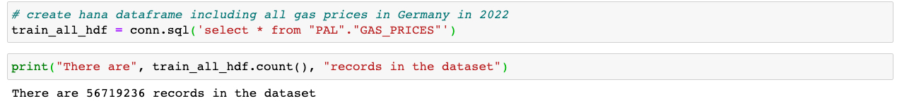
As preparation the data is downloaded as csv files from the 'tankerkönig' website and imported into the HANA database using the 'import Data' functionality in SAP HANA Database Explorer. We create one database for all the gas stations in Germany GAS_STATIONS and another table for the gas prices GAS_PRICES. There are 56 million records of gas prices alone for the current year, therefore we upload only those records, which must be done in several chunks of 1 GB.
Now, we can create a HANA dataframe in Python against the database table
Since our analysis will be limited to the area around SAP's headquarter in Walldorf, we filter the GAS_PRICES dataset for those stations located in the Rhein-Neckar area using HANA spatial functionality.
First, we need to upload the stations records, including the latitude and longitude information.
In order to spatially select the gas stations to those near SAP’s headquarter in Walldorf, we want to utilize spatial boundary information about the state of Baden-Württemberg, hence we upload a corresponding shapefile, which also contains the local districts shape information and can then perform a spatial join on the data.
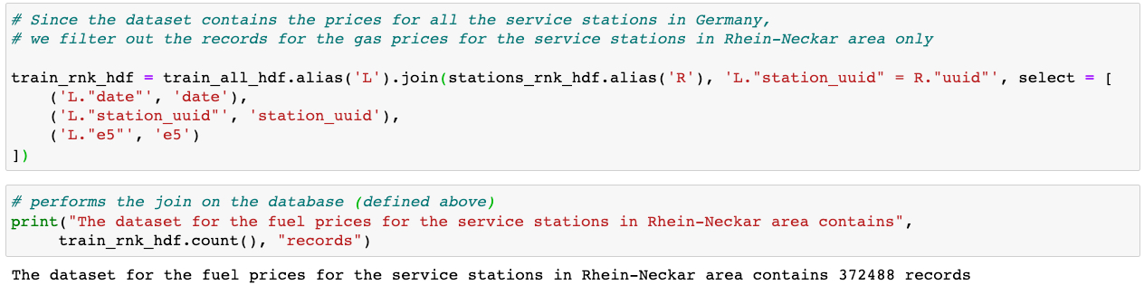
This reduces the number of service stations from over 15000 in Germany, to 2010 in Baden-Württemberg, to 111 in the Rhein-Neckar district.
As the last step in the data preparation phase, we join our dataset with all the gas price records in Germany with the gas stations located in the Rhein-Neckar district:
This dataset represents time series data starting from 2022-01-01 until 2022-06-21. Based on this dataset, we are creating three HANA dataframes:
Dataframe screenshot/code??
Very popular in these days among data scientist is a time series forecasting algorithm based on additive models also called prophet. Is proven to be very robust and usually provides good results even without extensive tuning of the hyperparameters. The Predictive Analysis Library (PAL) in SAP HANA has an optimized and very fast implementation of the algorithm called AdditiveModelAnalysis (link)
Now, we create an instance of the AdditiveModelForecast object and start the training of the forecast model (fit-method) by specifying the key, a group_key and holiday information (which here is an empty, dummy dataframe). As we want to train and execute a forecast model for each gas station in parallel, thus make use of segmented forecasting, we set the massive parameter as True and specify station-id as the group-key.
This will create a model, in fact, it will create one model for each service station in the dataset. We can now perform predictions and compare the results with the corresponding ground truth.
We pick one service station which is very close to SAP's headquarter in Walldorf and plot the results of the forecast calculations together with the historical price records.
When zooming in into the forecast results for the last seven day, we compare the predictions with the ground truth together with the confidence interval calculated by the prophet algorithm.
In case the forecast results meet the required accuracy requirements, the final step the data scientist needs to perform is handing over the corresponding design time artifacts to an application developer. Therefore, the HDI design time artifacts, most importantly the training and forecast procedures, need to be generated and made available, e.g., in a common git repository. From there, they can be easily consumed and used during the development of an intelligent application.
It is important to enable SQL tracing in the notebook before any ML training is carried out. Based on the information captured in traces, the HDI design time artifacts will be generated using the HANAGenerator method(link):
The last step generates the corresponding design time artifacts like grants, , synonyms, ... and most importantly the fit and predict procedures.
These artifacts can now be pushed into a git repository and the app developer can pull them into an app development project.
The complete notebook will be available on GitHub.
Note, beside the method of HDI artefact generation, the Python Machine Learning client also provides methods for each algorithm to inspect the executed SQL statements, like get_fit_execute_statement(), get_predict_execute_statement() and more, see Additive Model Forecast documentation for more details (link).

In this particular blog of the series, we focus on the data scientist's work, i.e., understanding the business problem, performing experiments, creating appropriate machine learning models and finally generating the corresponding design time artifacts. These artifacts can then be exchanged with the application developer by pushing/pulling them to a common git repository.
As a problem statement to illustrate the process, we want to forecast the gas prices at service stations within a region close to the SAP Headquarter in Germany, called the Rhein-Neckar district. Fortunately, a dataset is publicly available which can be used for our purpose.
The dataset is published on the public website “tankerkönig“ (http://www.tankerkoenig.de/). This dataset contains the gas prices of all gas stations in Germany from 2014 until today as csv files. A record contains the station id, the datetime, prices for diesel, e5 and e10 and a change indicator. In a separate csv the data of the service stations including its geolocation is provided.
Since we want to predict the gas prices simultaneously for various service stations, we conduct a segmented (or massive) time-series forecast. During this process, many machine learning models will be trained, in fact, one for each service station, which will then be used during the forecast calculations. Assuming that different geographical locations of service stations led to different usage patterns and eventually also have an impact on the gas price, we will calculate machine learning models for the individual service stations rather than using average calculations for groups of stations.
The focus in this blog post is not on developing the best machine learning model, but to demonstrate how to develop a reasonably good model with relative low effort using the capabilities of HANA ML and, in particular, the hana_ml python package.
Prerequisites
In the following we assume that you have an instance of SAP HANA Cloud available with at least three virtual CPUs. The SAP HANA database script server must be running (see HANA cloud central documentation), and you have a user which has been granted the appropriate rights to use the HANA PAL library (see documentation).
Import the required python packages
Start a Jupyter Notebook and import the required python packages. See this blog (link) for details on setting up your Python Machine Learning client for SAP HANA environment for use with SAP HANA Cloud.

Connect to the HANA Database

Load and explore datasets
As preparation the data is downloaded as csv files from the 'tankerkönig' website and imported into the HANA database using the 'import Data' functionality in SAP HANA Database Explorer. We create one database for all the gas stations in Germany GAS_STATIONS and another table for the gas prices GAS_PRICES. There are 56 million records of gas prices alone for the current year, therefore we upload only those records, which must be done in several chunks of 1 GB.
Now, we can create a HANA dataframe in Python against the database table
Since our analysis will be limited to the area around SAP's headquarter in Walldorf, we filter the GAS_PRICES dataset for those stations located in the Rhein-Neckar area using HANA spatial functionality.
First, we need to upload the stations records, including the latitude and longitude information.

In order to spatially select the gas stations to those near SAP’s headquarter in Walldorf, we want to utilize spatial boundary information about the state of Baden-Württemberg, hence we upload a corresponding shapefile, which also contains the local districts shape information and can then perform a spatial join on the data.

This reduces the number of service stations from over 15000 in Germany, to 2010 in Baden-Württemberg, to 111 in the Rhein-Neckar district.

As the last step in the data preparation phase, we join our dataset with all the gas price records in Germany with the gas stations located in the Rhein-Neckar district:
This dataset represents time series data starting from 2022-01-01 until 2022-06-21. Based on this dataset, we are creating three HANA dataframes:
- train_rnk_hdf - training data between 2022-01-01 and 2022-06-14
- test_rnk_hdf - test data starting from 2022-06-14 (gas prices set to zero)
- test_groundtruth_hdf - ground truth starting 2022-06-16 (with the original gas prices)
Dataframe screenshot/code??
Time series forecasting using Additive Model Time Series Analysis (prophet)
Very popular in these days among data scientist is a time series forecasting algorithm based on additive models also called prophet. Is proven to be very robust and usually provides good results even without extensive tuning of the hyperparameters. The Predictive Analysis Library (PAL) in SAP HANA has an optimized and very fast implementation of the algorithm called AdditiveModelAnalysis (link)
Now, we create an instance of the AdditiveModelForecast object and start the training of the forecast model (fit-method) by specifying the key, a group_key and holiday information (which here is an empty, dummy dataframe). As we want to train and execute a forecast model for each gas station in parallel, thus make use of segmented forecasting, we set the massive parameter as True and specify station-id as the group-key.

This will create a model, in fact, it will create one model for each service station in the dataset. We can now perform predictions and compare the results with the corresponding ground truth.

We pick one service station which is very close to SAP's headquarter in Walldorf and plot the results of the forecast calculations together with the historical price records.

When zooming in into the forecast results for the last seven day, we compare the predictions with the ground truth together with the confidence interval calculated by the prophet algorithm.
In case the forecast results meet the required accuracy requirements, the final step the data scientist needs to perform is handing over the corresponding design time artifacts to an application developer. Therefore, the HDI design time artifacts, most importantly the training and forecast procedures, need to be generated and made available, e.g., in a common git repository. From there, they can be easily consumed and used during the development of an intelligent application.
Generation of the HDI design time artifacts
It is important to enable SQL tracing in the notebook before any ML training is carried out. Based on the information captured in traces, the HDI design time artifacts will be generated using the HANAGenerator method(link):
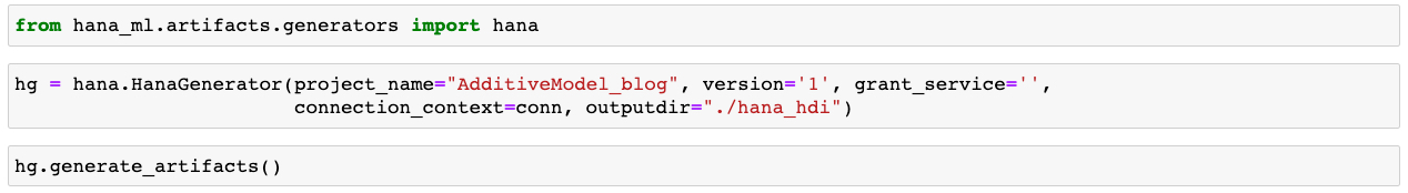
The last step generates the corresponding design time artifacts like grants, , synonyms, ... and most importantly the fit and predict procedures.

These artifacts can now be pushed into a git repository and the app developer can pull them into an app development project.
The complete notebook will be available on GitHub.
Note, beside the method of HDI artefact generation, the Python Machine Learning client also provides methods for each algorithm to inspect the executed SQL statements, like get_fit_execute_statement(), get_predict_execute_statement() and more, see Additive Model Forecast documentation for more details (link).
- SAP Managed Tags:
- Machine Learning,
- SAP HANA
Labels:
6 Comments
You must be a registered user to add a comment. If you've already registered, sign in. Otherwise, register and sign in.
Labels in this area
-
ABAP CDS Views - CDC (Change Data Capture)
2 -
AI
1 -
Analyze Workload Data
1 -
BTP
1 -
Business and IT Integration
2 -
Business application stu
1 -
Business Technology Platform
1 -
Business Trends
1,661 -
Business Trends
87 -
CAP
1 -
cf
1 -
Cloud Foundry
1 -
Confluent
1 -
Customer COE Basics and Fundamentals
1 -
Customer COE Latest and Greatest
3 -
Customer Data Browser app
1 -
Data Analysis Tool
1 -
data migration
1 -
data transfer
1 -
Datasphere
2 -
Event Information
1,400 -
Event Information
64 -
Expert
1 -
Expert Insights
178 -
Expert Insights
273 -
General
1 -
Google cloud
1 -
Google Next'24
1 -
Kafka
1 -
Life at SAP
784 -
Life at SAP
11 -
Migrate your Data App
1 -
MTA
1 -
Network Performance Analysis
1 -
NodeJS
1 -
PDF
1 -
POC
1 -
Product Updates
4,577 -
Product Updates
326 -
Replication Flow
1 -
RisewithSAP
1 -
SAP BTP
1 -
SAP BTP Cloud Foundry
1 -
SAP Cloud ALM
1 -
SAP Cloud Application Programming Model
1 -
SAP Datasphere
2 -
SAP S4HANA Cloud
1 -
SAP S4HANA Migration Cockpit
1 -
Technology Updates
6,886 -
Technology Updates
403 -
Workload Fluctuations
1
Related Content
- SAP HANA Cloud Vector Engine: Quick FAQ Reference in Technology Blogs by SAP
- 10+ ways to reshape your SAP landscape with SAP Business Technology Platform – Blog 4 in Technology Blogs by SAP
- SAP Successfactors Implementation and Maintenance in Projects in 2024 in Technology Blogs by Members
- Experiencing Embeddings with the First Baby Step in Technology Blogs by Members
- Harnessing the Power of SAP HANA Cloud Vector Engine for Context-Aware LLM Architecture in Technology Blogs by SAP
Top kudoed authors
| User | Count |
|---|---|
| 13 | |
| 10 | |
| 10 | |
| 7 | |
| 7 | |
| 6 | |
| 6 | |
| 5 | |
| 5 | |
| 4 |