

- SAP Community
- Products and Technology
- Technology
- Technology Blogs by SAP
- Dataiku triggering calculations / ML in SAP Data W...
Technology Blogs by SAP
Learn how to extend and personalize SAP applications. Follow the SAP technology blog for insights into SAP BTP, ABAP, SAP Analytics Cloud, SAP HANA, and more.
Turn on suggestions
Auto-suggest helps you quickly narrow down your search results by suggesting possible matches as you type.
Showing results for
Product and Topic Expert
Options
- Subscribe to RSS Feed
- Mark as New
- Mark as Read
- Bookmark
- Subscribe
- Printer Friendly Page
- Report Inappropriate Content
09-06-2022
12:56 PM
If Dataiku is part of your landscape, you might enjoy the option to use your familiar Dataiku environment to trigger data processing in your SAP Data Warehouse Cloud / SAP HANA Cloud systems.
Connect from Dataiku to the data in SAP Data Warehouse Cloud / SAP HANA Cloud and carry out data explorations, preparations, calculations, and Machine Learning. The data remains in place, thereby avoiding unnecessary data movement and data duplication. Save your outcomes as semantic views or physical tables. And if needed, you can still extract the data into Dataiku for further processing. However, you might not need to move all granular records, just the aggregated / prepared / filtered / predicted data that you require. Dataiku can then further process the data and write the outcomes back to SAP Data Warehouse Cloud / SAP HANA Cloud.
If you would like to stay instead within the SAP Business Technology Platform, you have the familiar choices to deploy your Python / R code with SAP Data Intelligence, CloudFoundry and Kyma. Either way, SAP’s Python package hana_ml and R package hana.ml.r make it easy to trigger such an advanced analysis from any Python or R environment on the data held in SAP Data Warehouse Cloud / SAP HANA Cloud.
In case this use case and blog is somewhat familiar to you, then you have probably already seen a related blog, which explains this scenario with Azure Machine Learning or Databricks as front end.
Let’s go through the different options with a time series forecast as example.
In this scenario we are assuming that you are working with SAP Data Warehouse Cloud. However, an implementation with SAP HANA Cloud would be very similar:
You also need to have access to a Dataiku environment with Enterprise features enabled. According to the Dataiku website, only their Enterprise plan allows Dataiku to connect to SAP HANA. This blog was written with the free Dataiku edition (virtual machine), which starts with a 14 day Enterprise trial. I suggest to reach out to both SAP as well as Dataiku to verify which of these scenarios are covered by your licenses.
Begin by creating a new environment, which has SAP's hana_ml library installed. Navigate in Dataiku to Applications -> Administration -> Code Envs and click "NEW PYTHON ENV".
Open the environment when it has been created. On the "Packages to install" tab add the following lines as "Requested package". It might look as if the box only takes a single line, but you can add multiple at once.
Then click "SAVE AND UPDATE" and the libraries get installed. shapely is a dependency of the hana_ml library, that we don’t actually use. The code in this blog would still work, but you would receive a warning that shapely is missing. So shapely is only installed here to avoid that warning.
Create a new blank project to use that new environment.
Create a new notebook in that project, using the option "Write your own".
In the following prompt:
The notebook opens up. It already contains a few cells with Python code. These are not needed in our scenario and can be deleted. Verify that the notebook can use the hana_ml library that was installed earlier. Run the following code and you should see the version of hana_ml displayed.
With the hana_ml library installed, you can establish a connection to the SAP Data Warehouse Cloud. Just enter your database user’s details as a quick test (see prerequisites above). This code should result with the output “True”, to confirm that the connection was created. Should this fail, you might still need to add the IP address of your cluster to the “IP Allowlist” in SAP Data Warehouse Cloud.
To keep the logon credentials more secure, store the password as user secret in Dataiku (User Center -> Profile and settings -> My Account -> Other credentials) and retrieve it by code.
Now logon without having to hard code the password.
In your own projects you might be working with data that is already in SAP Data Warehouse Cloud. To follow this blog's example, load some data into the system for us to work with. Load the Power consumption of Tetouan city Data Set from the UCI Machine Learning Repository into a pandas DataFrame. (Salam, A., & El Hibaoui, A. (2018, December). Comparison of Machine Learning Algorithms for the Power Consumption Prediction:-Case Study of Tetouan city“. In 2018 6th International Renewable and Sustainable Energy Conference (IRSEC) (pp. 1-5). IEEE).
The data shows the power consumption of the Moroccan city in 10-minute intervals for the year 2017. We will use the data to create a time series forecast.
Use the hana_ml library and the connection that you have already established, to load this data into SAP Data Warehouse Cloud. The table and the appropriate columns will be created automatically.
Create a hana_ml DataFrame, which points to the data that remains in SAP Data Warehouse Cloud. We will be using this object extensively. Its collect() method can return the data as pandas DataFrame. To have a peek at the data, just select 5 rows.
You can check on the column types.
Have SAP Data Warehouse Cloud calculate some statistics about the data content.
The above distribution statistics were all calculated in SAP Data Warehouse Cloud. Only the results were transferred to your notebook. You can see the SELECT statement that was created by the describe() method.
You can also request further calculations on the data, or use ready-made exploratory plots. Have SAP Data Warehouse Cloud calculate a correlation matrix on the granular data. As you would expect, there is for instance a fair positive correlation between temperature and power consumption.
Now plot part of the data’s time series. Download the records of the last 7 days and plot them locally. The calculation 6 * 24 * 7 specifies how many most recent rows we are interested in. The data is in 10-minute intervals, so 6 gets a full hour. Multiplied by 24 to get a day, multiplied by 7 to get one week. The power consumption clearly has a strong daily pattern.
For further analysis add a DATE and MONTH column. These columns are added logically to the hana_ml DataFrame. The original table remains unchanged. Not data gets duplicated.
With the MONTH column, we can now create a boxplot that shows how consumption changes through the year. August has the highest median consumption.
Let’s get ready for a daily forecast. Have SAP Data Warehouse Cloud aggregate the 10-minute intervals to daily aggregates. Save the aggregation logic as view in the SAP Data Warehouse Cloud and show a few of the aggregated rows. The view could come in handy if you want to create the forecast within Dataiku (see below in the blog) on aggregated data. You would have reduced the amount of data that needs to travel.
Plot the daily consumption of the last 3 weeks.
SAP Data Warehouse Cloud has an Automated ML framework built-in as well as 100+ individual algorithms. The hana_ml library’s documentation has all the details. For our time series forecast we choose to use an AdditiveModelForecast, which is an implementation of the Prophet algorithm, and train a model.
To create predictions, you just need to specify for which dates predictions should be produced. Use the historic data (on which the model was trained) to dynamically obtain a pandas DataFrame, which lists the future 21 dates, for which we want to create a prediction.
Bring this data through the hana_ml library as temporary table to SAP Data Warehouse Cloud.
Use the temporary table as input for the prediction.
With the prediction now available as hana_ml DataFrame, you are free to use the predictions as required by your use case. Download the predictions for instance into a pandas DataFrame and have them plotted. The weekly pattern is nicely represented.
Or look at the predictions, still from Dataiku. Here with the predicted columns renamed before the display.
Or save the predictions as table to SAP Data Warehouse Cloud, where SAP Analytics Cloud, or another tool of your choice could pick up the predictions to share them with a broader user base.
You have used Dataiku to explore data in SAP Data Warehouse Cloud, prepare the data, create a forecast and share the predictions to SAP Analytics Cloud. No data got duplicated along the way, thereby reducing architectural and governmental complexity. This logic can be further automated of course. The next part of this blog shows how to deploy that Python code in a Dataiku Flow, ie to regularly produce and share the latest predictions.
To deploy the above code for regular execution, go into the project's Flow, which is still empty.
No Dataiku dataset needs to be added, as no data will be loaded. The data processing will happen in SAP Data Warehouse Cloud. Therefore, add a recipe of type Code / Python.
The recipe will run the code required to carry out a forecast within SAP Data Warehouse Cloud and to save the forecast into a table in SAP Data Warehouse Cloud. This logic does not require Dataiku to pass any input into the logic. Dataiku requires a signal though, that the code has completed. Hence add an output named "terminationsignal" that will save a CSV file into Dataiku's managed filesystem. We will add a line to our code, so that a meaningless pandas DataFrame is returned.
Add the following code to the recipe to
Before running the code set the recipe's Python environment in the Advanced settings to our hanaml environment.
Now run the Flow and it's hana_ml code manually or schedule the execution for instance with a time-based trigger.
You can now sandbox and deploy the execution of Machine Learning in SAP Data Warehouse Cloud out of Dataiku.
In the above example the data stayed in SAP Data Warehouse Cloud and the forecast was created in SAP Data Warehouse itself. The following example shows, how the forecast can be calculated in Dataiku itself. Dataiku can request detailed or aggregated data from SAP Data Warehouse Cloud, create the forecast and write the predictions back to SAP Data Warehouse Cloud.
This setup requires the Dataiku connector for SAP HANA, which it appears, is only available with Dataiku Enterprise. The example in this blog was created with the free Edition of Dataiku, which provides the Enterprise functionality for 2 weeks.
In the above Python example the connection to SAP Data Warehouse Cloud was made with a Python script, using SAP's hana_ml package. In this example, you establish a connection to SAP Data Warehouse Cloud using Dataiku's connector to SAP HANA.
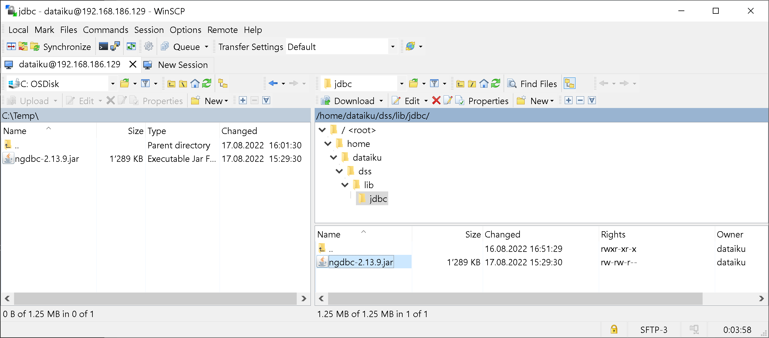
To create such a connection, the SAP HANA driver has to be installed on Dataiku. Download SAP HANA’s JDBC driver from SAP Development Tools (currently the file is called ngdbc-2.13.9.jar). Follow the Dataiku documentation Installing database drivers to add this driver to the system.
Personally, I found the installation steps to be slightly different to the documentation. Maybe the free virtual machine has some minor differences to the full product. The documentation recommends to stop the Dataiku Data Science Studio before copying the JDBC driver over. However, stopping the DSS always triggered an immediate restart. For me it worked to copy the driver into a running system, and to stop the system afterwards. After its automatic restart the driver was available.
Anyhow, you can copy the JDBC driver through SFTP, ie with WinSCP.
Copy the file over into the folder specified in the Dataiku documentation. On my system the path is home/dataiku/dss/lib/jdbc.
Now restart the Dataiku Data Science Server:
In case the Dataiku system does not restart automatically, bring it back up with
Now create a connection to SAP Data Warehouse Cloud: Go into: Applications -> Administration -> Connections -> NEW CONNECTION -> SAP Hana
Give the connection a name and enter your logon credentials. Test the connection and hit SAVE.
Create a new project to use this connection in a separate Flow. Now use Dataiku functionality to add either the table with the granular data ("POWERCONSUMPTION") or the view with the daily aggregates ("V_POWERCONSUMPTION_DAILY") as Dataset.
Then build the Flow using Dataiku's recipes as you require. In this example I am using a plugin for time series forecasting. The first recipe trains and saves the model. The second recipe picks up the saved model, creates a forecast and writes the predictions into a SAP HANA table.
This concludes the roundtrip. Dataiku downloaded data (possibly aggregated or prepared) from SAP Data Warehouse Cloud, created a forecast and wrote the predictions back to SAP Data Warehouse Cloud.
You got to know a couple of options to combine Dataiku with SAP Data Warehouse Cloud. Use Python to trigger calculations and Machine Learning in SAP Data Warehouse Cloud itself, keep the data where it is. Or download / upload the data to and from Dataiku as required.
Connect from Dataiku to the data in SAP Data Warehouse Cloud / SAP HANA Cloud and carry out data explorations, preparations, calculations, and Machine Learning. The data remains in place, thereby avoiding unnecessary data movement and data duplication. Save your outcomes as semantic views or physical tables. And if needed, you can still extract the data into Dataiku for further processing. However, you might not need to move all granular records, just the aggregated / prepared / filtered / predicted data that you require. Dataiku can then further process the data and write the outcomes back to SAP Data Warehouse Cloud / SAP HANA Cloud.
If you would like to stay instead within the SAP Business Technology Platform, you have the familiar choices to deploy your Python / R code with SAP Data Intelligence, CloudFoundry and Kyma. Either way, SAP’s Python package hana_ml and R package hana.ml.r make it easy to trigger such an advanced analysis from any Python or R environment on the data held in SAP Data Warehouse Cloud / SAP HANA Cloud.
In case this use case and blog is somewhat familiar to you, then you have probably already seen a related blog, which explains this scenario with Azure Machine Learning or Databricks as front end.

Let’s go through the different options with a time series forecast as example.
- Processing in SAP Data Warehouse Cloud through Python scripting in Dataiku:
- First use a Jupyter notebook in Dataiku to sandbox the scenario. Explore the data in SAP Data Warehouse Cloud, aggregate it and create a time series forecast on the aggregates. All triggered from Dataiku, executed in SAP Data Warehouse Cloud.
- Then deploy the final code as recipe in a graphical Dataiku Flow.
- Processing in Dataiku
- Download the aggregated data from SAP Data Warehouse Cloud into a Dataiku Flow, create a time series forecast within Dataiku and write the predictions to SAP Data Warehouse Cloud
Prerequisite
In this scenario we are assuming that you are working with SAP Data Warehouse Cloud. However, an implementation with SAP HANA Cloud would be very similar:
- You need access to a SAP Data Warehouse Cloud system with three virtual CPUs (free trial is not sufficient)
- The script server must be activated, see the documentation
- Create a Database User in your SAP Data Warehouse Cloud space, with the options “Enable Automated Predictive Library and Predictive Analysis Library”, “Enable Read Access” and “Enable Write Access” selected, see the documentation
- To trigger the Machine Learning in SAP Data Warehouse Cloud, you need that user’s password and the system’s host name, see this tutorial
You also need to have access to a Dataiku environment with Enterprise features enabled. According to the Dataiku website, only their Enterprise plan allows Dataiku to connect to SAP HANA. This blog was written with the free Dataiku edition (virtual machine), which starts with a 14 day Enterprise trial. I suggest to reach out to both SAP as well as Dataiku to verify which of these scenarios are covered by your licenses.
Python Scripting - Jupyter Notebook
Begin by creating a new environment, which has SAP's hana_ml library installed. Navigate in Dataiku to Applications -> Administration -> Code Envs and click "NEW PYTHON ENV".
- Name the environment: hanaml
- Leave "use conda" unselected.
- Click CREATE

Open the environment when it has been created. On the "Packages to install" tab add the following lines as "Requested package". It might look as if the box only takes a single line, but you can add multiple at once.
hana-ml==2.13.22072200

shapely
Then click "SAVE AND UPDATE" and the libraries get installed. shapely is a dependency of the hana_ml library, that we don’t actually use. The code in this blog would still work, but you would receive a warning that shapely is missing. So shapely is only installed here to avoid that warning.
Create a new blank project to use that new environment.
![]()
Create a new notebook in that project, using the option "Write your own".

In the following prompt:
- Select "PYTHON" as language
- Set "Code env" to hanaml (which is the environment we have just created)
- Name the notebook: DWC_Python
- Click CREATE

The notebook opens up. It already contains a few cells with Python code. These are not needed in our scenario and can be deleted. Verify that the notebook can use the hana_ml library that was installed earlier. Run the following code and you should see the version of hana_ml displayed.
import hana_ml

print(hana_ml.__version__)
With the hana_ml library installed, you can establish a connection to the SAP Data Warehouse Cloud. Just enter your database user’s details as a quick test (see prerequisites above). This code should result with the output “True”, to confirm that the connection was created. Should this fail, you might still need to add the IP address of your cluster to the “IP Allowlist” in SAP Data Warehouse Cloud.
import hana_ml.dataframe as dataframe

conn = dataframe.ConnectionContext(address='[YOURDBUSERSHOSTNAME]',

                                   port=443,

                                   user='[YOURDBUSER]',

                                   password='[YOURDBUSERSPASSWORD]')

conn.connection.isconnected()
To keep the logon credentials more secure, store the password as user secret in Dataiku (User Center -> Profile and settings -> My Account -> Other credentials) and retrieve it by code.
import dataiku

client = dataiku.api_client()

auth_info = client.get_auth_info(with_secrets=True)

for secret in auth_info["secrets"]:

        if secret["key"] == "DWC_password":

                DWC_password = secret["value"]

                break
Now logon without having to hard code the password.
import hana_ml.dataframe as dataframe

conn = dataframe.ConnectionContext(address='[YOURDBUSERSHOSTNAME]',

                                   port=443,

                                   user='[YOURDBUSER]',

                                   password=DWC_password)

conn.connection.isconnected()
In your own projects you might be working with data that is already in SAP Data Warehouse Cloud. To follow this blog's example, load some data into the system for us to work with. Load the Power consumption of Tetouan city Data Set from the UCI Machine Learning Repository into a pandas DataFrame. (Salam, A., & El Hibaoui, A. (2018, December). Comparison of Machine Learning Algorithms for the Power Consumption Prediction:-Case Study of Tetouan city“. In 2018 6th International Renewable and Sustainable Energy Conference (IRSEC) (pp. 1-5). IEEE).
The data shows the power consumption of the Moroccan city in 10-minute intervals for the year 2017. We will use the data to create a time series forecast.
import pandas as pd

df_data = pd.read_csv('https://archive.ics.uci.edu/ml/machine-learning-databases/00616/Tetuan%20City%20power%20consumption.csv')

df_data.columns = map(str.upper, df_data.columns)

df_data.columns = df_data.columns.str.replace(' ', '_')

df_data.DATETIME = pd.to_datetime(df_data.DATETIME)
Use the hana_ml library and the connection that you have already established, to load this data into SAP Data Warehouse Cloud. The table and the appropriate columns will be created automatically.
import hana_ml.dataframe as dataframe

df_remote = dataframe.create_dataframe_from_pandas(connection_context=conn,

                                                   pandas_df=df_data,

                                                   table_name='POWERCONSUMPTION',

                                                   force=True,

                                                   replace=False)
Create a hana_ml DataFrame, which points to the data that remains in SAP Data Warehouse Cloud. We will be using this object extensively. Its collect() method can return the data as pandas DataFrame. To have a peek at the data, just select 5 rows.
df_remote = conn.table('POWERCONSUMPTION')

df_remote.head(5).collect()
You can check on the column types.
df_remote.dtypes()
Have SAP Data Warehouse Cloud calculate some statistics about the data content.
df_remote.describe().collect()
The above distribution statistics were all calculated in SAP Data Warehouse Cloud. Only the results were transferred to your notebook. You can see the SELECT statement that was created by the describe() method.
print(df_remote.describe().select_statement)You can also request further calculations on the data, or use ready-made exploratory plots. Have SAP Data Warehouse Cloud calculate a correlation matrix on the granular data. As you would expect, there is for instance a fair positive correlation between temperature and power consumption.
import matplotlib.pyplot as plt

from hana_ml.visualizers.eda import EDAVisualizer

f = plt.figure()

ax1 = f.add_subplot(111) # 111 refers to 1x1 grid, 1st subplot

eda = EDAVisualizer(ax1)

ax, corr_data = eda.correlation_plot(data=df_remote, cmap='coolwarm')
Now plot part of the data’s time series. Download the records of the last 7 days and plot them locally. The calculation 6 * 24 * 7 specifies how many most recent rows we are interested in. The data is in 10-minute intervals, so 6 gets a full hour. Multiplied by 24 to get a day, multiplied by 7 to get one week. The power consumption clearly has a strong daily pattern.
df_data = df_remote.tail(n=6*24*7, ref_col='DATETIME').collect()

df_data.drop('DATETIME', axis=1).plot(subplots=True,

                                    figsize=(10, 14));
For further analysis add a DATE and MONTH column. These columns are added logically to the hana_ml DataFrame. The original table remains unchanged. Not data gets duplicated.
df_remote = conn.table('POWERCONSUMPTION')

df_remote = df_remote.select('*', ('TO_DATE(DATETIME)', 'DATE'))

df_remote = df_remote.select('*', ('LEFT(DATE, 7)', 'MONTH'))

df_remote.head(5).collect()
With the MONTH column, we can now create a boxplot that shows how consumption changes through the year. August has the highest median consumption.
import matplotlib.pyplot as plt

from hana_ml.visualizers.eda import EDAVisualizer

f = plt.figure()

ax1 = f.add_subplot(111) # 111 refers to 1x1 grid, 1st subplot

eda = EDAVisualizer(ax1)

ax, cont = eda.box_plot(data = df_remote,

                        column='ZONE_1_POWER_CONSUMPTION', groupby='MONTH', outliers=True)

ax.legend(bbox_to_anchor=(1, 1));
Let’s get ready for a daily forecast. Have SAP Data Warehouse Cloud aggregate the 10-minute intervals to daily aggregates. Save the aggregation logic as view in the SAP Data Warehouse Cloud and show a few of the aggregated rows. The view could come in handy if you want to create the forecast within Dataiku (see below in the blog) on aggregated data. You would have reduced the amount of data that needs to travel.
df_remote_daily = df_remote.agg([('sum', 'ZONE_1_POWER_CONSUMPTION', 'ZONE_1_POWER_CONSUMPTION_SUM')], group_by='DATE')

df_remote_daily.save('V_POWERCONSUMPTION_DAILY')

df_remote_daily.head(5).collect()
Plot the daily consumption of the last 3 weeks.
df_data = df_remote_daily.tail(n=21, ref_col='DATE').collect()


import matplotlib.pyplot as plt

from matplotlib.pyplot import figure

figure(figsize=(12, 5))

plt.plot(df_data['DATE'], df_data['ZONE_1_POWER_CONSUMPTION_SUM'])

plt.xticks(rotation=45);
SAP Data Warehouse Cloud has an Automated ML framework built-in as well as 100+ individual algorithms. The hana_ml library’s documentation has all the details. For our time series forecast we choose to use an AdditiveModelForecast, which is an implementation of the Prophet algorithm, and train a model.
from hana_ml.algorithms.pal.tsa.additive_model_forecast import AdditiveModelForecast

amf = AdditiveModelForecast(growth='linear')

amf.fit(data=df_remote_daily.select('DATE', 'ZONE_1_POWER_CONSUMPTION_SUM'))
To create predictions, you just need to specify for which dates predictions should be produced. Use the historic data (on which the model was trained) to dynamically obtain a pandas DataFrame, which lists the future 21 dates, for which we want to create a prediction.
import pandas as pd

strLastDate = str( df_remote_daily.select('DATE').max())

df_topredict = pd.date_range(strLastDate, periods=1 + 21, freq="D", closed='right').to_frame()

df_topredict.columns = ['DATE']

df_topredict['DUMMY'] = 0

df_topredict
Bring this data through the hana_ml library as temporary table to SAP Data Warehouse Cloud.
import hana_ml.dataframe as dataframe

df_rem_topredict = dataframe.create_dataframe_from_pandas(connection_context=conn,

                                                   pandas_df=df_topredict,

                                                   table_name='#TOPREDICTDAILY',

                                                   force=True,

                                                   replace=False)
Use the temporary table as input for the prediction.
df_rem_predicted = amf.predict(data=df_rem_topredict)With the prediction now available as hana_ml DataFrame, you are free to use the predictions as required by your use case. Download the predictions for instance into a pandas DataFrame and have them plotted. The weekly pattern is nicely represented.
df_data = df_rem_predicted.collect()


from matplotlib import pyplot as plt

figure(figsize=(12, 5))

plt.plot(df_data['DATE'], df_data['YHAT'])

plt.fill_between(df_data['DATE'],df_data['YHAT_LOWER'], df_data['YHAT_UPPER'], alpha=.3)

plt.xticks(rotation=45);
Or look at the predictions, still from Dataiku. Here with the predicted columns renamed before the display.
df_rem_predicted = df_rem_predicted.rename_columns(['DATE', 'PREDICTION', 'PREDICTION_LOWER', 'PREDICTION_UPPER'])

df_rem_predicted.collect()
Or save the predictions as table to SAP Data Warehouse Cloud, where SAP Analytics Cloud, or another tool of your choice could pick up the predictions to share them with a broader user base.
df_rem_predicted.save('POWERCONSUMPTION_21DAYPRED', force=True)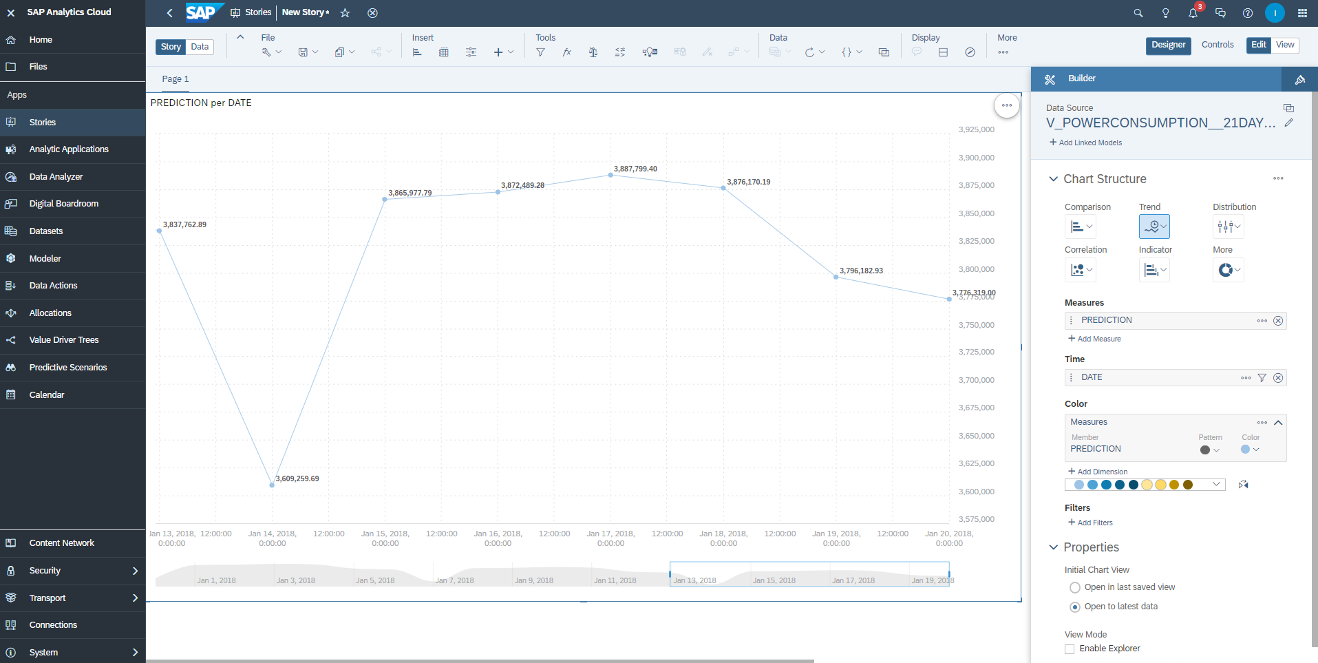
You have used Dataiku to explore data in SAP Data Warehouse Cloud, prepare the data, create a forecast and share the predictions to SAP Analytics Cloud. No data got duplicated along the way, thereby reducing architectural and governmental complexity. This logic can be further automated of course. The next part of this blog shows how to deploy that Python code in a Dataiku Flow, ie to regularly produce and share the latest predictions.
Python Scripting - Deployment
To deploy the above code for regular execution, go into the project's Flow, which is still empty.
![]()
No Dataiku dataset needs to be added, as no data will be loaded. The data processing will happen in SAP Data Warehouse Cloud. Therefore, add a recipe of type Code / Python.

The recipe will run the code required to carry out a forecast within SAP Data Warehouse Cloud and to save the forecast into a table in SAP Data Warehouse Cloud. This logic does not require Dataiku to pass any input into the logic. Dataiku requires a signal though, that the code has completed. Hence add an output named "terminationsignal" that will save a CSV file into Dataiku's managed filesystem. We will add a line to our code, so that a meaningless pandas DataFrame is returned.

Add the following code to the recipe to
- retrieve the password for SAP Data Warehouse Cloud from Dataiku's credential store
- create a forecast in SAP Data Warehouse Cloud
- save the forecast to a table in SAP Data Warehouse Cloud
- send a pandas DataFrame at the end to signal the completion to the Dataiku Flow
# Get DWC password

import dataiku

client = dataiku.api_client()

auth_info = client.get_auth_info(with_secrets=True)

for secret in auth_info["secrets"]:

        if secret["key"] == "DWC_password":

                DWC_password = secret["value"]

                break


# Logon to DWC

import hana_ml.dataframe as dataframe

conn = dataframe.ConnectionContext(address='c71cde07-f86a-4258-b92a-55aff26c9044.hana.prod-eu10.hanacloud.ondemand.com',

                                   port=443,

                                   user='DWCDATA#DWCDBUSER',

                                   password=DWC_password)

conn.connection.isconnected()


# Prepare the data

df_remote = conn.table('POWERCONSUMPTION')

df_remote = df_remote.select('*', ('TO_DATE(DATETIME)', 'DATE'))

df_remote_daily = df_remote.agg([('sum', 'ZONE_1_POWER_CONSUMPTION', 'ZONE_1_POWER_CONSUMPTION_SUM')], group_by='DATE')


# Train the forecasting model

from hana_ml.algorithms.pal.tsa.additive_model_forecast import AdditiveModelForecast

amf = AdditiveModelForecast(growth='linear')

amf.fit(data=df_remote_daily.select('DATE', 'ZONE_1_POWER_CONSUMPTION_SUM'))


# Determine which dates to forecast

import pandas as pd

strLastDate = str( df_remote_daily.select('DATE').max())

df_topredict = pd.date_range(strLastDate, periods=1 + 21, freq="D", closed='right').to_frame()

df_topredict.columns = ['DATE']

df_topredict['DUMMY'] = 0


# Forecast those dates

import hana_ml.dataframe as dataframe

df_rem_topredict = dataframe.create_dataframe_from_pandas(connection_context=conn,

                                                   pandas_df=df_topredict,

                                                   table_name='#TOPREDICTDAILY',

                                                   force=True,

                                                   replace=False)

df_rem_predicted = amf.predict(data=df_rem_topredict)


# Save the forecasts to SAP Data Warehouse Cloud

df_rem_predicted.save('POWERCONSUMPTION_21DAYPRED', force=True)


# Send termination signal

terminationsignal_df = pd.DataFrame(['DONE'], columns=['SIGNAL'])
Before running the code set the recipe's Python environment in the Advanced settings to our hanaml environment.

Now run the Flow and it's hana_ml code manually or schedule the execution for instance with a time-based trigger.
You can now sandbox and deploy the execution of Machine Learning in SAP Data Warehouse Cloud out of Dataiku.
Processing in Dataiku
In the above example the data stayed in SAP Data Warehouse Cloud and the forecast was created in SAP Data Warehouse itself. The following example shows, how the forecast can be calculated in Dataiku itself. Dataiku can request detailed or aggregated data from SAP Data Warehouse Cloud, create the forecast and write the predictions back to SAP Data Warehouse Cloud.
This setup requires the Dataiku connector for SAP HANA, which it appears, is only available with Dataiku Enterprise. The example in this blog was created with the free Edition of Dataiku, which provides the Enterprise functionality for 2 weeks.
Step 1 of 2 for Dataiku processing: Install the SAP HANA driver
In the above Python example the connection to SAP Data Warehouse Cloud was made with a Python script, using SAP's hana_ml package. In this example, you establish a connection to SAP Data Warehouse Cloud using Dataiku's connector to SAP HANA.
To create such a connection, the SAP HANA driver has to be installed on Dataiku. Download SAP HANA’s JDBC driver from SAP Development Tools (currently the file is called ngdbc-2.13.9.jar). Follow the Dataiku documentation Installing database drivers to add this driver to the system.
Personally, I found the installation steps to be slightly different to the documentation. Maybe the free virtual machine has some minor differences to the full product. The documentation recommends to stop the Dataiku Data Science Studio before copying the JDBC driver over. However, stopping the DSS always triggered an immediate restart. For me it worked to copy the driver into a running system, and to stop the system afterwards. After its automatic restart the driver was available.
Anyhow, you can copy the JDBC driver through SFTP, ie with WinSCP.

Copy the file over into the folder specified in the Dataiku documentation. On my system the path is home/dataiku/dss/lib/jdbc.
Now restart the Dataiku Data Science Server:
- Log into the operating system of Dataiku's virtual machine. The user and password are displayed on the screen.
- Stop the Data Science Studio with:
cd dss

cd bin

./dss stop
In case the Dataiku system does not restart automatically, bring it back up with
./dss startNow create a connection to SAP Data Warehouse Cloud: Go into: Applications -> Administration -> Connections -> NEW CONNECTION -> SAP Hana
Give the connection a name and enter your logon credentials. Test the connection and hit SAVE.

Step 2 of 2 for Dataiku processing: Implement
Create a new project to use this connection in a separate Flow. Now use Dataiku functionality to add either the table with the granular data ("POWERCONSUMPTION") or the view with the daily aggregates ("V_POWERCONSUMPTION_DAILY") as Dataset.

Then build the Flow using Dataiku's recipes as you require. In this example I am using a plugin for time series forecasting. The first recipe trains and saves the model. The second recipe picks up the saved model, creates a forecast and writes the predictions into a SAP HANA table.

This concludes the roundtrip. Dataiku downloaded data (possibly aggregated or prepared) from SAP Data Warehouse Cloud, created a forecast and wrote the predictions back to SAP Data Warehouse Cloud.
Summary
You got to know a couple of options to combine Dataiku with SAP Data Warehouse Cloud. Use Python to trigger calculations and Machine Learning in SAP Data Warehouse Cloud itself, keep the data where it is. Or download / upload the data to and from Dataiku as required.
Labels:
2 Comments
You must be a registered user to add a comment. If you've already registered, sign in. Otherwise, register and sign in.
Labels in this area
-
ABAP CDS Views - CDC (Change Data Capture)
2 -
AI
1 -
Analyze Workload Data
1 -
BTP
1 -
Business and IT Integration
2 -
Business application stu
1 -
Business Technology Platform
1 -
Business Trends
1,658 -
Business Trends
91 -
CAP
1 -
cf
1 -
Cloud Foundry
1 -
Confluent
1 -
Customer COE Basics and Fundamentals
1 -
Customer COE Latest and Greatest
3 -
Customer Data Browser app
1 -
Data Analysis Tool
1 -
data migration
1 -
data transfer
1 -
Datasphere
2 -
Event Information
1,400 -
Event Information
66 -
Expert
1 -
Expert Insights
177 -
Expert Insights
294 -
General
1 -
Google cloud
1 -
Google Next'24
1 -
Kafka
1 -
Life at SAP
780 -
Life at SAP
13 -
Migrate your Data App
1 -
MTA
1 -
Network Performance Analysis
1 -
NodeJS
1 -
PDF
1 -
POC
1 -
Product Updates
4,577 -
Product Updates
340 -
Replication Flow
1 -
RisewithSAP
1 -
SAP BTP
1 -
SAP BTP Cloud Foundry
1 -
SAP Cloud ALM
1 -
SAP Cloud Application Programming Model
1 -
SAP Datasphere
2 -
SAP S4HANA Cloud
1 -
SAP S4HANA Migration Cockpit
1 -
Technology Updates
6,873 -
Technology Updates
419 -
Workload Fluctuations
1
Related Content
- New Machine Learning features in SAP HANA Cloud in Technology Blogs by SAP
- What’s New in SAP Analytics Cloud Release 2024.07 in Technology Blogs by SAP
- SAP Datasphere - Space, Data Integration, and Data Modeling Best Practices in Technology Blogs by SAP
- Porting Legacy Data Models in SAP Datasphere in Technology Blogs by SAP
- Recap — SAP Data Unleashed 2024 in Technology Blogs by Members
Top kudoed authors
| User | Count |
|---|---|
| 35 | |
| 25 | |
| 14 | |
| 7 | |
| 7 | |
| 6 | |
| 6 | |
| 5 | |
| 4 | |
| 4 |