

- SAP Community
- Products and Technology
- Technology
- Technology Blogs by SAP
- Carbon Emission Forecasting: How SAP Analytics Clo...
Technology Blogs by SAP
Learn how to extend and personalize SAP applications. Follow the SAP technology blog for insights into SAP BTP, ABAP, SAP Analytics Cloud, SAP HANA, and more.
Turn on suggestions
Auto-suggest helps you quickly narrow down your search results by suggesting possible matches as you type.
Showing results for
Product and Topic Expert
Options
- Subscribe to RSS Feed
- Mark as New
- Mark as Read
- Bookmark
- Subscribe
- Printer Friendly Page
- Report Inappropriate Content
09-01-2022
11:23 AM
Introduction
Global warming poses a serious threat to all human beings. Especially the record-breaking heatwaves have swept across the northern hemisphere during the summer, making developing carbon emission reduction strategies across all industries imperative.
To lower carbon emissions, businesses need to investigate the historical data and try to gain insights into future emissions. So, can SAP Analytics Cloud help businesses to better understand their carbon emission data and provide insightful advice on how to reduce their emission? Yes for sure!
In this blog, we take advantage of the prediction planning feature of SAP Analytics Cloud to show the trend of carbon emissions in China based on 20 years of real-world data.
You will learn:
- How to build a planning model based on historical carbon emission data.
- How to use "influencing factors" in time series prediction to further optimize the prediction results.
- How to conduct a "What-If" simulation with different assumptions.
Scenario and Dataset
We used a public dataset containing carbon emissions and macroeconomic data for China from 1998 to 2019. This dataset includes many independent variables that may affect carbon emissions, for example, the GDP of different industries, urbanization ratio, total exports, highway mileage, total thermal power generation, population, etc. We used this dataset to create a planning model and generate carbon emissions predictions for the next five years (2020 to 2025).
For predictions, We purposed three scenarios and predicted the carbon emissions accordingly: baseline mode (BM), high growth mode (HGM), and sustainable growth mode (SGM). In the BM scenario, economic, social, and energy development will be carried out according to the national macro plan, and it will be used as the benchmark scenario. The HGM scenario assumes that China will continue the high-speed development. The SGM scenario is just the opposite, in which China will slow down its development to achieve more aggressive carbon-reduction goals.
Data Import and Build a Planning Model
First, we need to build a planning model to support the prediction. We select the “from a CSV or Excel File” from Modeler to build the planning model from our CSV data file, as shown in the figure below:

After importing, click "Enable Planning" and select "Year" as the planning date dimension to create the model. As shown in the following figure:

Now the creation of the planning model is completed. Next, we will create a time series prediction based on the planning model.
Prediction
Time series prediction can help users estimate and get prepared for future trends. In some cases, the target value to be predicted is only time-dependent, so accurate prediction can be achieved by using historical values only. However, sometimes the target value we want to predict depends not only on time but also on some other external factors. For example, the number of carbon emissions may be related to the season, government policies, or the total amount of thermal power plants.
Therefore, in SAP Analytics Cloud, we take advantage of the "influencing factors" feature when generating time series prediction model. “Influencing factors” allow the model to take external influences that affect the growth of a key figure into account, which leads to more accurate prediction results. Next, we will show you how to use the "influencing factors" feature to improve the accuracy of prediction.
Baseline Model
Let's create a "baseline" prediction model to predict carbon emissions without using influencing factors. We will predict the amount of carbon emission for one prediction point (2019). based on the 21 years of historical data (1998-2018) , We select "regions" as entities to predict the number of carbon emissions for each province separately, as shown in the figure below.


We also configure a window size of 21 years, up to 2018.
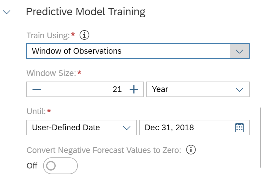
We didn’t add any influencing factor in this case.

After the training, we can draw the following conclusions from the prediction modeling report (as shown in the figure):
- The average expected MAPE of prediction is 4.88%;
- Different provinces have different prediction results, and the top and bottom (best and worst) entities are listed in the prediction report;
- Different entities (provinces) can be selected in the interpretation to obtain different prediction results.


The prediction results show that carbon emissions are related to time to some extent. But we want to introduce other influencing factors and test whether we can get better results.
Using influencing factors to improve the prediction model
We want to keep the baseline model as a reference and use the same settings for the new prediction model, so let's first duplicate the previous baseline model.

Open the newly created prediction model and scroll down to the "influencing factors" section in the settings. Let's test our hypothesis about the impact of macroeconomic variables on carbon emissions by adding the following influencing factors and training the prediction model:
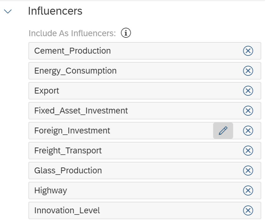

A time series prediction model can add up to 20 influencing factors. After the training, in the prediction modeling report, we draw the following conclusions:
- The average expected MAPE of prediction is 4.53%. Compared with the baseline model, the fitting of the model is improved;
- The top and bottom entities have changed. For example, without the influencing factors, the prediction result of Shanghai is poor. the prediction result of Shanghai has been improved with the help of influencing factors, which shows that Shanghai's carbon emissions are closely related to the macroeconomy;
- For Shanghai, the variables that have a greater impact on carbon emissions are thermal power generation, population, and cement production.


We will take Shanghai as an example to show the readers the follow-up workflow

In order to understand the "true" accuracy of the model, we need to check the accuracy of the horizontal period. By magnifying the visualization results of prediction and reality, we can see that for Shanghai, when using influencing factors, the prediction sequence is closer to the actual time series:


Furthermore, if we only use the above three influencing factors to predict again,as shown in the following figure:

After the model training, in the prediction modeling report, we draw the following conclusions:
- The average expected MAPE of prediction is 4.09%. Compared with adding all the influencing factors, the fitting of the model is further improved;
- The top entity and the bottom entities changed again;
- The model fitting results of each entity are optimized.


Some influencing factors we selected in the setting didn’t appear in the list. The prediction model only retains "useful" influencing factors. It evaluates additional performance gain introduced b each influencing factor, and uses only those that bring enough positive effects on the results. Therefore, it is important to understand that if an influencing factor does not significantly improve the prediction accuracy, it is impossible to force the prediction model to use the influencing factor.
Next, we will use the three influencing factors to conduct what-if simulations based on different policy scenarios to predict future carbon emissions in China.
What-if Simulation
We introduced the concept and related knowledge of what-if simulation in the previous blog. If you are not familiar with how to use SAP Analytics Cloud for what-if analysis, it is recommended to read this blog ( link) first.
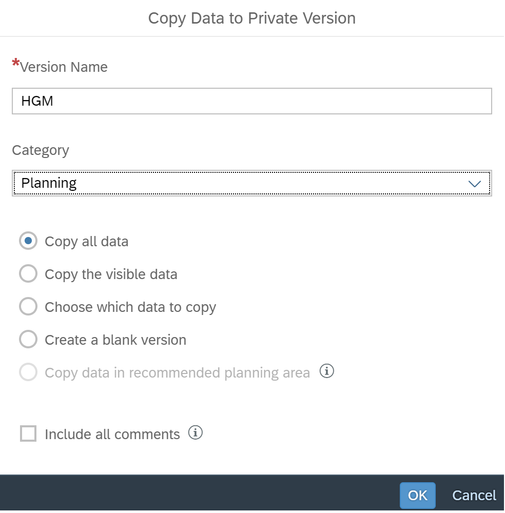
We have introduced and defined three scenarios: HGM, BM, and SGM. We use separated planning versions for each simulation scenario. In the SAP analytics cloud, prediction models can be trained and applied to a single version each time, not multiple versions. Therefore, first, we need to create three versions by copying all the data of the actual version.
First, we will enter the version management to create private versions of the three scenarios, as shown in the figure below.


For the three scenarios, we only pay attention to the three selected influencing factors that affect the prediction results in the above prediction model, namely thermal power generation, population, and cement production. We take Shanghai as an example. For each scenario, we used the following growth rates for each influencing factor:
| Scenarios | Population | Thermal_Power | Cement_Production |
| HGM | 0.5% | -8% | 10% |
| BM | 0.4% | -10% | 6% |
| SGM | 0.3% | -12% | -1% |
Next, we will train the prediction model. Now we will duplicate the time series prediction model that only contains the above three influencing factors, and use the following settings to create the first prediction model for HGM (we only consider Shanghai as the prediction entity):


We use the same settings for the other two prediction models. Before the training, we use the "duplicate" function to duplicate the model and change the planning version.
Now we have three trained models that can generate predictions for three different scenarios. We only need to write the forecast results of each model back to different versions.

Now we are ready to visualize the simulation results in a story as shown below.

Now we have the carbon emission prediction for 2020-2025 under the three scenarios of HGM, BM, and SGM. Based on the prediction, no matter which mode of development will be adopted in Shanghai in the future, the amount of carbon emission shows a downward trend, and the decline rate is the fastest under the mode of sustainable development.
Conclusion
In this blog post, we used real-world carbon emission data as an example to demonstrate how to use SAP Analytics Cloud to build prediction models and perform what-if simulations. You’re welcome to try it out and generate your own predictions for your hometown.
If you would like to learn more about Predictive Planning:
- You can also explore our learning track.
- You can also go hands-on and experience SAP Analytics Cloud by yourself.
Full Credits: Stephen Hong
- SAP Managed Tags:
- SAP Analytics Cloud,
- SAP Analytics Cloud, augmented analytics
Labels:
2 Comments
You must be a registered user to add a comment. If you've already registered, sign in. Otherwise, register and sign in.
Labels in this area
-
ABAP CDS Views - CDC (Change Data Capture)
2 -
AI
1 -
Analyze Workload Data
1 -
BTP
1 -
Business and IT Integration
2 -
Business application stu
1 -
Business Technology Platform
1 -
Business Trends
1,658 -
Business Trends
91 -
CAP
1 -
cf
1 -
Cloud Foundry
1 -
Confluent
1 -
Customer COE Basics and Fundamentals
1 -
Customer COE Latest and Greatest
3 -
Customer Data Browser app
1 -
Data Analysis Tool
1 -
data migration
1 -
data transfer
1 -
Datasphere
2 -
Event Information
1,400 -
Event Information
66 -
Expert
1 -
Expert Insights
177 -
Expert Insights
293 -
General
1 -
Google cloud
1 -
Google Next'24
1 -
Kafka
1 -
Life at SAP
780 -
Life at SAP
13 -
Migrate your Data App
1 -
MTA
1 -
Network Performance Analysis
1 -
NodeJS
1 -
PDF
1 -
POC
1 -
Product Updates
4,577 -
Product Updates
340 -
Replication Flow
1 -
RisewithSAP
1 -
SAP BTP
1 -
SAP BTP Cloud Foundry
1 -
SAP Cloud ALM
1 -
SAP Cloud Application Programming Model
1 -
SAP Datasphere
2 -
SAP S4HANA Cloud
1 -
SAP S4HANA Migration Cockpit
1 -
Technology Updates
6,873 -
Technology Updates
417 -
Workload Fluctuations
1
Related Content
- SAP Sustainability Footprint Management: Q1-24 Updates & Highlights in Technology Blogs by SAP
- What’s New in SAP Analytics Cloud Release 2024.07 in Technology Blogs by SAP
- Unleashing AI and Machine Learning in Sales: Advanced Price-Volume Forecasting with SAP Analytics Cl in Technology Blogs by SAP
- Predictive Forecast Disaggregation in Technology Blogs by SAP
- Recap — SAP Data Unleashed 2024 in Technology Blogs by Members
Top kudoed authors
| User | Count |
|---|---|
| 35 | |
| 25 | |
| 13 | |
| 7 | |
| 7 | |
| 6 | |
| 6 | |
| 6 | |
| 5 | |
| 4 |