
- SAP Community
- Products and Technology
- Supply Chain Management
- SCM Blogs by SAP
- How to Take Advantage of Machine Learning Forecast...
Supply Chain Management Blogs by SAP
Expand your SAP SCM knowledge and stay informed about supply chain management technology and solutions with blog posts by SAP. Follow and stay connected.
Turn on suggestions
Auto-suggest helps you quickly narrow down your search results by suggesting possible matches as you type.
Showing results for
Advisor
Options
- Subscribe to RSS Feed
- Mark as New
- Mark as Read
- Bookmark
- Subscribe
- Printer Friendly Page
- Report Inappropriate Content
10-27-2021
10:01 AM

Hi there!
I am a Product Manager for SAP Integrated Business Planning for demand at SAP and I am here to share some insights on how to leverage SAP IBP machine learning capabilities.
Let’s assume you are a demand planner who knows that the forecast of your product(s) does not depend only on the sales history, but it is influenced by other external factors. Let’s say you are interested in knowing which are the factors that influence your forecast, what is their importance and what is their impact.
Then you are in the right place! You can take advantage of the Machine Learning capabilities of SAP IBP for demand (available now!), based on the forecasting algorithms included in the Predictive Analytics Library (PAL) of SAP.
In particular, the algorithm we are interested in is Hybrid Gradient Boosting of Decision Trees (HGBDT).
Let’s have a short deep dive in the algorithm.
Gradient Boosting of Decision Trees – a short explanation
Gradient Boosting of Decision Trees is an ensemble machine learning technique for regression and classification problems.
Let me shortly explain what “Decision Trees” and “Gradient Boosting” stand for.
A decision tree is a tree-like graph in which each internal node represents a “test” on an attribute (e.g. whether a coin flip comes up heads or tails), each branch represents the outcome of the test, and each leaf node represents the actual output/decision taken (or class label).
Decision trees belong to a class of supervised machine learning algorithms, which are used in both classification (predicts discrete outcome) and regression (predicts continuous numeric outcomes) predictive modeling.
The goal of the algorithm is to predict a target variable from a set of input variables and their attributes. The approach builds a tree structure through a series of binary splits (yes/no) from the root node via branches passing several decision nodes (internal nodes), until we come to leaf nodes. Source
Decision trees are called “weak learner”, because the predictions made by a single decision tree are better than a random method but still not very accurate.
Therefore the need for “Gradient Boosting”.
In statistical terms boosting is a method of additive modelling designed to provide a better predictive performance by combining multiple simple models together. In this case, Gradient Boosting takes the results of multiple decision trees, and looks to reduce the errors from each iteration sequentially to create a “stronger”, more complex predictor. A robust predictive model is therefore built by the linear addition of multiple decision trees, i.e. “Boosted”. Source
If you are already an expert on Gradient Boosting and would like more details on how it is implemented in SAP’s PAL see the official Help page.
Variable Impact Analysis – how it works
When using HGBDT to forecast a product in SAP IBP for demand, multiple things happen.
The Gradient Boosting algorithm first learns how the independent variables affected the sales in the past (even considering the combination of variables).

Then the forecast will be generated based on these learnings.
The forecast generation is independent from the variable impact analysis.
If the variable impact analysis is required, then the forecast (let’s call it total forecast from now on) will be split into a baseline forecast (including trend and seasonality) and impact key figures (for those of you who are not familiar with SAP IBP, consider key figure to a be a synonym of time series).

Baseline and impact key figures can also be defined for Ex-Post forecast.
You can choose the same key figure for more than one variable if you wish (then the impact of the variables will be summed up).
If no impact key figure is defined for a variable, the impact calculated for it is added to the baseline forecast or baseline ex-post forecast.
Small technical comment: if you choose the same baseline key figure for the forecast and the ex-post forecast, you should also choose the same impact key figure for them.
In the following example I am going to use the independent variables also mentioned in the image above: Marketing Budget, Product Price and Calendar Events (for which I use a categorical key figure), and corresponding impact key figures Marketing Budget Impact, Product Price Impact and Event Impact.
How to set up a forecast model with HGBDT in SAP IBP for demand
In the following I will assume you are familiar with the SAP Integrated Business Planning solution and therefore you already know how to set up a planning area, planning objects, key figures, application jobs, application job templates etc.
If you are not familiar with this, you may understand the content only partly, but this may not bring a lot of value for you (so I suggest to stop reading here!).
So let’s get started….
Moving forward I assume the following conditions have already been met:
- Historical data (sales history) has been gathered
- Historical data (sales history) has been cleansed.
- Independent (external) variable data is already present in SAP IBP (as already mentioned before I will be using marketing budget, product price and a categorical key figure for calendar events).
- Impact key figures have been defined (in the following example they are Marketing Budget Impact, Product Price Impact, event Impact)
Go to “Manage Forecast Models” and create a new model.
In general section decide a name and the granularity of the forecast together with the number of weeks that should be considered in the past and in the future.

Add any preprocessing steps you might need. Please consider that with Gradient Boosting correcting outliers might be counterproductive, as they may be due to the impact of an independent variable and removing them could hinder the learning process of the algorithm.
Note: if you use preprocessing step Outlier Correction with Outlier Correction Method "No correction" (i.e. the system identifies the outliers but does nothing about them), then IBP can generate a feature called "Periods with outliers" that can be consumed by HGBT.

In the “Forecasting Steps” tab select input key figures (sales history) and output key figures (total forecast).
Then select “Gradient Boosting of Decision Trees” as an algorithm.
At this point you already need to know which external variables are of potential interest in the computation of the forecast. You can add them in the “Independent Variables” section.
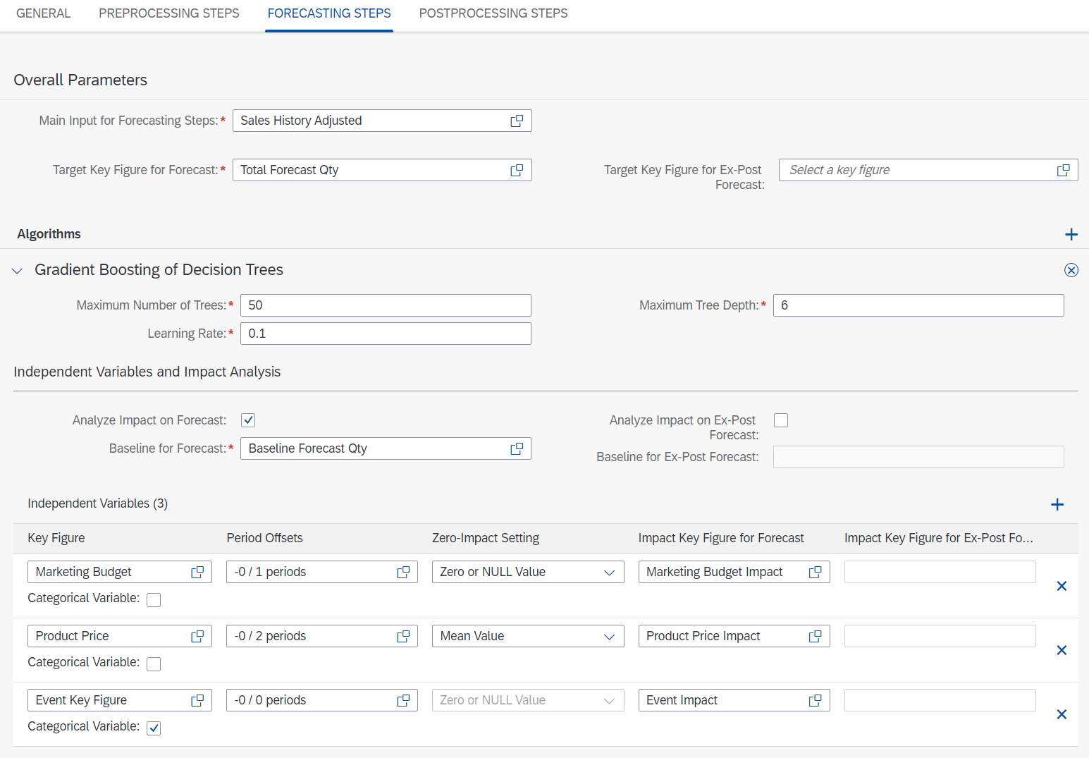
In this example I want to analyze the impact of the variables.
As explained in the previous section, this is not a must: you could also just use Gradient Boosting to compute your forecast using the independent variables without variable impact analysis. In this case the Gradient Boosting algorithm will still take the independent variables into consideration when generating the forecast, but you would not be able to see how they affected the generated forecast.
If you do decide to analyze the impact of the key figures, however, you have to check the box “Analyze Impact on Forecast” and define impact key figures for this purpose. For non-categorical variables you also need to define the Zero-Impact Setting.
To complete the settings of the model, add any additional post-processing steps you need.

Finally, save the model.
The Zero-Impact Setting
The Zero-Impact Setting will have a big effect on the variable impact analysis: this setting should represent the “usual” value of the variable you are considering.
In my example, the marketing budget is usually zero, and only from time to time some budget is allocated. Then the expectation is that whenever the budget is zero there is not impact on the sales, but when it is positive the sales will change.
For the product price (again, referring to my example) it is different: the price of a product is never expected to be zero. Rather, it will have an average value, and whenever the price varies from the average sales are affected.
For this reason in this case the Zero-Impact Setting is not zero but rather the mean value.
Run Statistical Forecasting Job from Fiori or Excel
You can run the Forecasting Job from Fiori or through the SAP IBP Excel Add-in.
In the log you can see the importance of the external variables:

And after running the job this is how your forecast could look like:

I would like to highlight once more that one of the strengths of HGBDT, compared to other multivariate algorithms like MLR or ARIMAX, is that it is able to estimate the combined impact of multiple independent variables.
For example, let's assume you have two independent variables. Then HGBDT is able to find out that if any of the two variables, then sales increase as well, but if both of them increase at the same time, then sales drop.
So that was it! I hope this helped you gain some insights into the Machine Learning capabilities of SAP IBP for demand.
Go and try it out yourself!
Find out more:
- SAP Integrated Business Planning I Demand Planning
- Intelligent Forecasting with Machine Learning in SAP IBP (video)
- SAP IBP Overview
- SAP IBP Community
- Roadmaps
- SAP Customer Influence Portal for SAP IBP
- Questions? Ask here
- SAP Managed Tags:
- SAP Integrated Business Planning for Supply Chain
Labels:
11 Comments
You must be a registered user to add a comment. If you've already registered, sign in. Otherwise, register and sign in.
Labels in this area
-
Business Trends
169 -
Business Trends
24 -
Catalog Enablement
1 -
Event Information
47 -
Event Information
4 -
Expert Insights
12 -
Expert Insights
38 -
intelligent asset management
1 -
Life at SAP
63 -
Product Updates
500 -
Product Updates
66 -
Release Announcement
1 -
SAP Digital Manufacturing for execution
1 -
Super Bowl
1 -
Supply Chain
1 -
Sustainability
1 -
Swifties
1 -
Technology Updates
187 -
Technology Updates
17
Related Content
- “Mind the Gap” – Improves ROI, Cost & Margin by Merging Planning Processes in Supply Chain Management Blogs by SAP
- RISE with SAP advanced asset and service management package in Supply Chain Management Blogs by SAP
- SAP IBP: Enhancing Forecast Accuracy with Time Series Analysis and Change Point Detection in Supply Chain Management Blogs by SAP
- SAP Integrated Business Planning for Supply Chain (SAP IBP) 2402 - Available Now! in Supply Chain Management Blogs by SAP
- SAP Best Practices for SAP Integrated Business Planning for Supply Chain – 2402 in Supply Chain Management Blogs by SAP
Top kudoed authors
| User | Count |
|---|---|
| 10 | |
| 8 | |
| 6 | |
| 4 | |
| 4 | |
| 3 | |
| 3 | |
| 3 | |
| 3 | |
| 2 |