
- SAP Community
- Products and Technology
- Supply Chain Management
- SCM Blogs by Members
- Planning Multiple Deliveries in IBP using CPI-DS
Supply Chain Management Blogs by Members
Learn about SAP SCM software from firsthand experiences of community members. Share your own post and join the conversation about supply chain management.
Turn on suggestions
Auto-suggest helps you quickly narrow down your search results by suggesting possible matches as you type.
Showing results for
former_member76
Discoverer
Options
- Subscribe to RSS Feed
- Mark as New
- Mark as Read
- Bookmark
- Subscribe
- Printer Friendly Page
- Report Inappropriate Content
09-02-2021
8:13 AM
Business Context
Businesses often tend to split their orders from suppliers into multiple deliveries. The reason for doing this could be:
For e.g., the actual requirement for the next month production is 1000 units, however all the units may not be required when the production starts at the beginning of the month but sometime during the middle of the month. Say 500 units are required at the beginning of the month and the rest 500 need to be delivered by 14th of the month for the next production batch.
Doing this enables businesses to place a single order to suppliers with multiple line items corresponding to quantity required on each date. This also allows for suppliers to plan for their own production in advance.
Section 1: Use Case - Overview
A particular use case for this approach is when the business is doing forward planning for procuring material over the next 1-2 months. To get a visibility of the order quantity with delivery dates, the net requirement at a vendor level should also have a date attribute assigned to the planning level. This will help in directly releasing purchase requisition quantities from IBP along with the delivery dates.
Now to get the quantity at a delivery date level, we need two main inputs:
For e.g today is 10th January and PO is planned to be released. The lead time for a material from vendor is 20 days and the delivery offset is 10 days. Therefore, the delivery dates would be calculated as:
Delivery Date 1: Today + 20 Days OR 10th January + 20 days = 30th January
Delivery Date 2: Delivery Date 1 + Delivery Offset OR 30th January + 10 Days = 9th February
Now we will look into the configuration aspect of modelling the delivery split within IBP.
Section 2: Configuration
Step 1:
Introduce the attributes for Delivery Offset (Type Integer), Delivery Date 1 and Delivery Date 2 (Type Timestamp).
(Note: Since lead time is already a standard attribute in IBP, there is no need to create it separately.)
Assign these new attributes to the Location Source Master corresponding to the planning area and assign them to the planning area.
Create attribute Delivery Date and a new Master Data Type Delivery Date Master. The root attributes for this master data type will be Product ID, Location ID, Ship from Location ID and Delivery Date.
Assign the Delivery Date attribute to the planning area.
Step 2:
Load the values for Lead Time and Delivery Offset for each Product-Location-Vendor combination. Initial one-time load followed by delta loads whenever there are new planning combinations.
Step 3:
(Note that this step is outside IBP and the assumption is that communication is already setup between IBP and source systems through an integration interface)
Since IBP does not support calculation of attribute values, we will use another approach to calculate the values of delivery date 1 and delivery date 2 which will also help maintain the timestamp status of these attributes.
We will make use of the existing integration interface to complete this action. While the code will not be discussed, the basic outline of the logic is as follows:
Step 4:
The next step would be creating planning levels which include the delivery date attributes. Three main planning levels would be:
Step 5:
Create following new Key Figures
Configure the calculations as follows:
Delivery Qty 1 @ Prod-Loc-LocFr-DD1 = Net Requirement 1 @ Prod-Loc-Locfr * Delivery Qty 1 @ Prod-Loc-LocFr-DD1
Delivery Qty 2 @ Prod-Loc-LocFr-DD1 = Net Requirement 2 @ Prod-Loc-Locfr * Delivery Qty 2 @ Prod-Loc-LocFr-DD1
Note: Net Requirement 1 and Net Requirement 2 are the Key Figures which hold the delivery qty values at Product – Location – Vendor level post the split. They can be as simple as a fixed percentage of Net Requirement or other calculation logics can be used.
Here we use a simple logic wherein,
Net Requirement 1 @ Prod-Loc-Locfr = 0.5 * Net Requirement @ Prod-Loc-Locfr
Net Requirement 2 @ Prod-Loc-Locfr = 0.5 * Net Requirement @ Prod-Loc-Locfr
Step 6:
Since Delivery Qty 1 Helper and Delivery Qty 2 Helper are both stored key figures, the values need to be loaded for these. We will first understand the purpose of these key figures.
In IBP, to go from a less granular to more granular planning level the two methods are:
In this case we want to calculate delivery qty at a more granular level (Product – Location – Ship from Location – Delivery Date 1 / 2) than the planning level of net requirement (Product – Location – Ship from Location).
To achieve this, we will make use of the helper key figures by loading value 1 for all active combinations.
To load the values in these key figures, we will use the Location Source Master as a reference and once again leverage Cloud Platform Integration to pull the combinations in a flat file, default the values to 1 and load it into both key figures in the current bucket.
This automated process would need to run daily in the morning to update the delivery dates w.r.t current date.
Step 7:
Now that we have the data for the helpers, the Delivery Qty Key Figures will also get calculated dynamically. However, the quantities would be in two different key figures.
So, in the last step we will again use cloud platform integration to merge these key figures into a single key figure called PR Qty at the Product – Location – Ship from Location – Delivery Date Planning Level.
Prior to loading the key figure values, one must note that since each Product – Location – Vendor combination has 2 delivery dates, 2 unique line items would be required and for that, the delivery date too needs to be a root attribute. This is where the Delivery Date Master and the planning level Product – Location – Ship from Location – Delivery Date come into play.
The values in Delivery Date Master are loaded through a scheduled integration job using the Location Source Master as a reference and mapping both Delivery Date 1 and Delivery Date 2 (source attributes) to the Delivery Date (target attribute).
The values in PR Qty Key Figure are loaded through a user executed integration job using the Delivery Qty 1 and Delivery Qty 2 Key Figures as reference and mapping both Delivery Date 1 and Delivery Date 2 (source attributes) to the Delivery Date (target attribute).
As we can see, the PR Qty is known along with visibility of the delivery dates and this output can be directly sent to ECC for raising the POs with expected delivery timelines.
Apart from giving a visibility of the delivery dates it can also be used to monitor the compliance from the vendors by comparing the actual delivery dates with expected ones and determining how much quantity was received in time and how many were delayed.
In this way we are able to plan for multiple delivery dates on the same PO within SAP IBP by leveraging CPI-DS and then send this data to ERP system for directly raising PO with expected Delivery Dates from vendors, thereby eliminating the need to manually create POs in ERP system every time.
-----------------------------------------------------------X--------------------------------------------------------------------
Businesses often tend to split their orders from suppliers into multiple deliveries. The reason for doing this could be:
- Meeting transportation lot size requirements
- Reducing the unnecessary build-up of inventory and holding costs
- Freshness of batch in some cases
For e.g., the actual requirement for the next month production is 1000 units, however all the units may not be required when the production starts at the beginning of the month but sometime during the middle of the month. Say 500 units are required at the beginning of the month and the rest 500 need to be delivered by 14th of the month for the next production batch.
Doing this enables businesses to place a single order to suppliers with multiple line items corresponding to quantity required on each date. This also allows for suppliers to plan for their own production in advance.
Section 1: Use Case - Overview
A particular use case for this approach is when the business is doing forward planning for procuring material over the next 1-2 months. To get a visibility of the order quantity with delivery dates, the net requirement at a vendor level should also have a date attribute assigned to the planning level. This will help in directly releasing purchase requisition quantities from IBP along with the delivery dates.

Fig 1. Illustration of Delivery Split with Delivery Date
Now to get the quantity at a delivery date level, we need two main inputs:
- Average Lead Time for the vendor - The lead time will define the minimum number of days w.r.t day of PO release for the 1st order to be received.
- The number of days between the 1st and 2nd delivery – this will facilitate creating the second line item of the PO wherein date of 2nd delivery can be specified. (We will call this as ‘Delivery Offset’)
For e.g today is 10th January and PO is planned to be released. The lead time for a material from vendor is 20 days and the delivery offset is 10 days. Therefore, the delivery dates would be calculated as:
Delivery Date 1: Today + 20 Days OR 10th January + 20 days = 30th January
Delivery Date 2: Delivery Date 1 + Delivery Offset OR 30th January + 10 Days = 9th February

Fig 2. Calculation of Delivery Dates
Now we will look into the configuration aspect of modelling the delivery split within IBP.
Section 2: Configuration
Step 1:
Introduce the attributes for Delivery Offset (Type Integer), Delivery Date 1 and Delivery Date 2 (Type Timestamp).
(Note: Since lead time is already a standard attribute in IBP, there is no need to create it separately.)
Assign these new attributes to the Location Source Master corresponding to the planning area and assign them to the planning area.
Create attribute Delivery Date and a new Master Data Type Delivery Date Master. The root attributes for this master data type will be Product ID, Location ID, Ship from Location ID and Delivery Date.
Assign the Delivery Date attribute to the planning area.
Step 2:
Load the values for Lead Time and Delivery Offset for each Product-Location-Vendor combination. Initial one-time load followed by delta loads whenever there are new planning combinations.
Step 3:
(Note that this step is outside IBP and the assumption is that communication is already setup between IBP and source systems through an integration interface)
Since IBP does not support calculation of attribute values, we will use another approach to calculate the values of delivery date 1 and delivery date 2 which will also help maintain the timestamp status of these attributes.
We will make use of the existing integration interface to complete this action. While the code will not be discussed, the basic outline of the logic is as follows:
- Create a flow with Location Source as source table and flat file as target
- Create calculation expressions for the Delivery Date 1 and Delivery Date 2 columns
- Back integrate the newly created flat file into IBP Location Source with respective mappings

Fig 3. Location Source Master prior to Delivery Date Calculation

Fig 4. Location Source Master after Delivery Date Calculation
Step 4:
The next step would be creating planning levels which include the delivery date attributes. Three main planning levels would be:
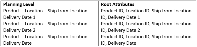
Fig 5. New Planning Levels with Root Attributes
Step 5:
Create following new Key Figures

Fig 6. New Key Figures with Base Planning Levels
Configure the calculations as follows:
Delivery Qty 1 @ Prod-Loc-LocFr-DD1 = Net Requirement 1 @ Prod-Loc-Locfr * Delivery Qty 1 @ Prod-Loc-LocFr-DD1
Delivery Qty 2 @ Prod-Loc-LocFr-DD1 = Net Requirement 2 @ Prod-Loc-Locfr * Delivery Qty 2 @ Prod-Loc-LocFr-DD1
Note: Net Requirement 1 and Net Requirement 2 are the Key Figures which hold the delivery qty values at Product – Location – Vendor level post the split. They can be as simple as a fixed percentage of Net Requirement or other calculation logics can be used.
Here we use a simple logic wherein,
Net Requirement 1 @ Prod-Loc-Locfr = 0.5 * Net Requirement @ Prod-Loc-Locfr
Net Requirement 2 @ Prod-Loc-Locfr = 0.5 * Net Requirement @ Prod-Loc-Locfr
Step 6:
Since Delivery Qty 1 Helper and Delivery Qty 2 Helper are both stored key figures, the values need to be loaded for these. We will first understand the purpose of these key figures.
In IBP, to go from a less granular to more granular planning level the two methods are:
- Copy to another Key Figure and Disaggregate to lower level
- Multiply by a Key Figure at the lower level
In this case we want to calculate delivery qty at a more granular level (Product – Location – Ship from Location – Delivery Date 1 / 2) than the planning level of net requirement (Product – Location – Ship from Location).
To achieve this, we will make use of the helper key figures by loading value 1 for all active combinations.
To load the values in these key figures, we will use the Location Source Master as a reference and once again leverage Cloud Platform Integration to pull the combinations in a flat file, default the values to 1 and load it into both key figures in the current bucket.
This automated process would need to run daily in the morning to update the delivery dates w.r.t current date.

Fig 7. Location Source Master Data

Fig 8. Key Figure Data for Delivery Qty 1 Helper

Fig 9. Key Figure Data for Delivery Qty 2 Helper
Step 7:
Now that we have the data for the helpers, the Delivery Qty Key Figures will also get calculated dynamically. However, the quantities would be in two different key figures.

Fig 10. Illustration of Delivery Qty Calculation for one combination
So, in the last step we will again use cloud platform integration to merge these key figures into a single key figure called PR Qty at the Product – Location – Ship from Location – Delivery Date Planning Level.
Prior to loading the key figure values, one must note that since each Product – Location – Vendor combination has 2 delivery dates, 2 unique line items would be required and for that, the delivery date too needs to be a root attribute. This is where the Delivery Date Master and the planning level Product – Location – Ship from Location – Delivery Date come into play.
The values in Delivery Date Master are loaded through a scheduled integration job using the Location Source Master as a reference and mapping both Delivery Date 1 and Delivery Date 2 (source attributes) to the Delivery Date (target attribute).

Fig 11. Delivery Date Master Data
The values in PR Qty Key Figure are loaded through a user executed integration job using the Delivery Qty 1 and Delivery Qty 2 Key Figures as reference and mapping both Delivery Date 1 and Delivery Date 2 (source attributes) to the Delivery Date (target attribute).

Fig 12. Creation of Purchase Requisition with Multiple Line Items
As we can see, the PR Qty is known along with visibility of the delivery dates and this output can be directly sent to ECC for raising the POs with expected delivery timelines.
Apart from giving a visibility of the delivery dates it can also be used to monitor the compliance from the vendors by comparing the actual delivery dates with expected ones and determining how much quantity was received in time and how many were delayed.
In this way we are able to plan for multiple delivery dates on the same PO within SAP IBP by leveraging CPI-DS and then send this data to ERP system for directly raising PO with expected Delivery Dates from vendors, thereby eliminating the need to manually create POs in ERP system every time.
-----------------------------------------------------------X--------------------------------------------------------------------
1 Comment
You must be a registered user to add a comment. If you've already registered, sign in. Otherwise, register and sign in.
Labels in this area
-
aATP
1 -
ABAP Programming
1 -
Activate Credit Management Basic Steps
1 -
Adverse media monitoring
1 -
Alerts
1 -
Ausnahmehandling
1 -
bank statements
1 -
Bin Sorting sequence deletion
1 -
Bin Sorting upload
1 -
BP NUMBER RANGE
1 -
Brazil
1 -
Business partner creation failed for organizational unit
1 -
Business Technology Platform
1 -
Central Purchasing
1 -
Charge Calculation
2 -
Cloud Extensibility
1 -
Compliance
1 -
Controlling
1 -
Controlling Area
1 -
Data Enrichment
1 -
DIGITAL MANUFACTURING
1 -
digital transformation
1 -
Dimensional Weight
1 -
Direct Outbound Delivery
1 -
E-Mail
1 -
ETA
1 -
EWM
6 -
EWM - Delivery Processing
2 -
EWM - Goods Movement
4 -
EWM Outbound configuration
1 -
EWM-RF
1 -
EWM-TM-Integration
1 -
Extended Warehouse Management (EWM)
3 -
Extended Warehouse Management(EWM)
7 -
Finance
1 -
Freight Settlement
1 -
Geo-coordinates
1 -
Geo-routing
1 -
Geocoding
1 -
Geographic Information System
1 -
GIS
1 -
Goods Issue
2 -
GTT
2 -
IBP inventory optimization
1 -
inbound delivery printing
1 -
Incoterm
1 -
Innovation
1 -
Inspection lot
1 -
intraday
1 -
Introduction
1 -
Inventory Management
1 -
Localization
1 -
Logistics Optimization
1 -
Map Integration
1 -
Material Management
1 -
Materials Management
1 -
MFS
1 -
New Feature
1 -
Outbound with LOSC and POSC
1 -
Packaging
1 -
PPF
1 -
PPOCE
1 -
PPOME
1 -
print profile
1 -
Process Controllers
1 -
Production process
1 -
QM
1 -
QM in procurement
1 -
Real-time Geopositioning
1 -
Risk management
1 -
S4 HANA
1 -
S4 HANA 2022
1 -
S4-FSCM-Custom Credit Check Rule and Custom Credit Check Step
1 -
S4SCSD
1 -
Sales and Distribution
1 -
SAP DMC
1 -
SAP ERP
1 -
SAP Extended Warehouse Management
2 -
SAP Hana Spatial Services
1 -
SAP IBP IO
1 -
SAP MM
1 -
sap production planning
1 -
SAP QM
1 -
SAP REM
1 -
SAP repetiative
1 -
SAP S4HANA
1 -
SAP TM
1 -
SAP Transportation Management
3 -
SAP Variant configuration (LO-VC)
1 -
SD (Sales and Distribution)
1 -
Source inspection
1 -
Storage bin Capacity
1 -
Supply Chain
1 -
Supply Chain Disruption
1 -
Supply Chain for Secondary Distribution
1 -
Technology Updates
1 -
TMS
1 -
Transportation Cockpit
1 -
Transportation Management
2 -
Visibility
2 -
warehouse door
1 -
WOCR
1
- « Previous
- Next »
Related Content
- SAP Intelligent Clinical Supply Management goes CTS Europe 2024 – our key insights in Supply Chain Management Blogs by SAP
- RISE with SAP Advanced Logistics Package in Supply Chain Management Blogs by SAP
- SAP Field Logistics: Centralized Supplier Item Repository for an Optimized Rental Process in Supply Chain Management Blogs by SAP
- Drive productivity, safely and sustainably, with SAP manufacturing solutions in Supply Chain Management Blogs by SAP
- SAP Transportation Management Analytics in Supply Chain Management Blogs by SAP
Top kudoed authors
| User | Count |
|---|---|
| 4 | |
| 3 | |
| 3 | |
| 2 | |
| 2 | |
| 2 | |
| 1 | |
| 1 | |
| 1 | |
| 1 |