
- SAP Community
- Products and Technology
- Technology
- Technology Blogs by SAP
- Augment your Python Analysis with Multi-Model data...
Technology Blogs by SAP
Learn how to extend and personalize SAP applications. Follow the SAP technology blog for insights into SAP BTP, ABAP, SAP Analytics Cloud, SAP HANA, and more.
Turn on suggestions
Auto-suggest helps you quickly narrow down your search results by suggesting possible matches as you type.
Showing results for
Advisor
Options
- Subscribe to RSS Feed
- Mark as New
- Mark as Read
- Bookmark
- Subscribe
- Printer Friendly Page
- Report Inappropriate Content
07-21-2021
12:02 PM
A lot of data science and machine learning work is done in Python. For this, the “Python machine learning client for SAP HANA” (hana-ml for short) provides easy access to SAP HANA tables in the form of Pandas compatible data-frames. However, with its multi-model capabilities (like spatial, graph, and document store), SAP HANA has more to offer. In this blog post, you will learn about the enhancements of the library to support these multi-model capabilities and how you can leverage them for your work. We will walk through an end-to-end example based on Wellington's stormwater network. We will evaluate and visualize the graph and show how we can analyze problems that might occur in the network based on built in graph algorithms. The data and code is available on github.com. If you want to run the Jupyter Notebook yourself, you need to take care about the prerequisites.
Credits to sascha.kiefer who implemented the multi-model extensions in hana-ml and created the Jupyter Notebook.
We use a separate JSON file to store database logon data...
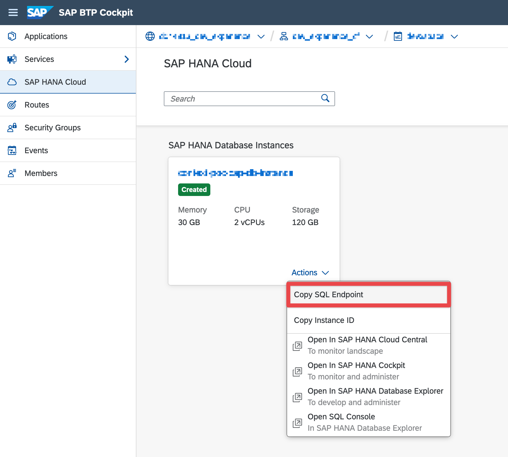
... the Notebook loads the logon information from this file, so we don't have to put them into the notebook itself. The database URL can be optained from the BTP Cockpit:
First, we import the libraries we need to create a connection to the database.
Next, we create a connection context, that represents the physical connection to your SAP HANA database instance. This connection context is used in the subsequent code to let the hana-ml library know where to connect to. The ConnectionContext is part of the hana-ml library.
Once the connection is set up, we create a Graph Workspace (in the subsequent text referred to as 'graph') based on imported vertices and edges in SAP HANA. As a result, we have the stormwater network stored as a graph in SAP HANA and we can run network analysis processes.
The hana-ml library offers different functions to create a graph:
A hana_ml.dataframe.DataFrame represents a database query as a data-frame (which is conceptually similar to a Pandas data-frame). Thus, it seamlessly fits into the toolset a data scientist is used to. The HANA DataFrame is designed to not bring data back from the database unless explicitly requested (lazy evaluation). That means all operations (like column filter, where clauses, ...) are performed on the query level, and only if certain methods (like collect()) are called, the data gets materialized and transferred to the client. All materialized data are returned as Pandas data-frames so that they can directly be used for further processing. The hana-ml library also provides functions to create data-frames from local data and store this data to a SAP HANA database table. Check out the hana_ml.dataframe documentation for further details. For our example, the data-frame's geospatial support becomes handy. During the data import, we can already specify which columns from our source are geometries. When we query the data and use them on the client, the geometries from database tables are directly converted to objects, which can be used in GeoPandas or other spatial libraries. As we will see, these geometries can be directly used with geospatial functions on the database layer.
In our example we create the graph from two CSV files – the data in one file represents the edges, i.e. the actual pipe segments, the other file contains the data for the pipe segment’s junctions. We use Pandas to import the data.
So, we execute create_dataframe_from_pandas() function of the hana-ml library to upload the data from a Pandas data-frame to SAP HANA and store it in a database table. It's worth mentioning, that we make use of the spatial features here already. The datasets include a SHAPE column, containing the spatial data in a Well-Known-Text format. hana-ml can directly convert WKT columns to geometries. This results in a column with the suffix _GEO (in our example SHAPE_GEO) in the table. You could even generate a geometry out of longitude and latitude columns. See the hana-ml function documentation for further details. Once the data is in SAP HANA, we create the graph in HANA.
The discover_graph_workspaces(cc) function displays all the graphs available in your database instance. So, you can check if the graph was created. The function returns something like this.
KeplerGl is a popular framework to visualize geospatial data. We use it in our example to display the stormwater network we're working with.
We already created the g_storm object above, so the following step is optional. It just shows how you would create a graph object representation in python from an existing graph workspace in SAP HANA.
Next, we run print(g_storm) and get some technical information about the graph. You specifically see the database tables the graph is based on and the columns that are used to define the source and target vertices of the edges.
The next statements bring up a map to visualize our stormwater network.
This is what happens:
g_storm.edges_hdf: the graph object provides direct access to several graph properties. The most important ones are edges_hdf and vertices_hdf, which both represent a HANA data-frame referring to the respective table in the database. In this example, we use the edges data-frame of our graph.
.select('ID', ('SHAPE_GEO.ST_TRANSFORM(4326).ST_ASGEOJSON()', 'GJ')) a HANA data-frame provides the select method as a filter on the columns you want to query. It can also be used to create new calculated columns on the fly. In this example we create a column GJ that is based on the column SHAPE_GEO (remember, that this was automatically generated as a geometry, when we imported the CSV data). First, we transform the data into the SRS 4326 (which is the spatial reference system expected by Kepler for visualization - remember our source data used the SRS 2193). Then we transform the data into GeoJSON format which can be interpreted by Kepler directly. This results in a data-frame with two columns: ID an GJ. The calculated column is not persisted to the database. Its lifespan is restricted to the lifespan of the data-frame object. However you could save() the data-frame to a HANA catalog object (either a new table or a view - see the API documentation for further details)
.collect() this method materializes the data of the HANA data-frame and transfers it to the client. Data is returned as a Pandas data-frame
The hana-ml library provides functionality to analyze and process the graph. In this section, we explore some of them.
The function g_storm.describe() gives you statistical information about the graph (e.g. counts, min-, max-values, density). In our example, we focus on IS_CONNECTED, which indicates that we don't have a single connected network, but multiple unconnected ones.
The hana-ml library provides algorithms, that can be executed on the graph (like shortest path, neighbors, topological sort, weakly connected components). They can be found in the hana_ml.graph.algorithms package. The execution pattern is always the same:
Every algorithm is implemented in a separate Python class which you can instantiate (<algorithm_name>). This class expects the graph instance as a constructor parameter (graph = <graph_instance>), so it knows on which graph to perform the algorithms. Finally, every algorithm class implements an execute() method, which triggers the execution of the algorithm. The result gives you access to the results of the algorithm execution. The properties available depend on the algorithm you execute.
In our case, we can use the WeaklyConnectedComponents algorithm to identify parts of our network - each weakly connected component represents a sub-graph, that is not connected to the other components.
The result indicates that we have 8332 independent components in the graph. Let's take a look at the number of vertices in each component.
Since components is a Pandas data-frame, we use Pandas capabilities to return only the two largest components - 25 and 5. With wcc.vertices the algorithm provides a data-frame that maps each vertex to the component it belongs to. Let's store the components to SAP HANA and use the subgraph() method of the graph for our visualization. We use the same method to upload the data to SAP HANA we used when we created the graph. The following statement stores the algorithm results to HANA.
As we have seen, the components 25 and 5 are the biggest ones in the graph. Let’s put them on a map to gain further insights. The Graph object provides a method to create subgraphs based on filter criteria on vertices or edges.
This creates a new graph with the name LM_STORMWATER_COMP1 based on a vertex filter. The filter selects only vertices from the components we persisted in the step before and which belong to component 25. In other words, we now have a new graph, i.e. vertices and edges that belong to component 25. We do the same for the vertices of component 5.
Like before, we use Kepler to visualize the two largest weakly connected components.
In this section, we evaluate how one could analyze which sections of our water network could cause a problem reported on a specific access point (i.e. vertex). We look at Neighbors, NeigborsSubgraphs and ShortestPath algorithms.
Let's assume somebody reported a problem with the node WCC_SW002719 (e.g. there is less flow than expected which might indicate a broken pipe somewhere else). We want to analyze that further. First, let's load the vertex itself. We use the same mechanisms we already used before. Since we want to map it later, we materialize the geo-location as a GeoJSON string.
Let's use the Neighbors algorithm to find all neighbors to our reported vertex and display the 5 closest:
If we want to plot the vertices on the map, we need to read the geometries from the database. For that we use the filter() method of the HANA data-frame.
With that we query and materialize all the geo-locations of all vertices which are 5 hops away from our start vertex. Now we plot the "problem" node and its neighbors.
The image above only shows the vertices reachable within 5 hops from the start vertex. However, when we want to find out what's the root cause of our reported problem, we need to identify all connected vertices. The water network is a directed graph, which means, we're only interested in upstream nodes, because if we see an issue on a node (e.g. less flow than expected), the root cause must be somewhere upstream (i.e. incoming to the node we're looking at). So instead of individual points let's look at subgraphs again.
This creates a subgraph starting from a given vertex and only evaluates incoming edges (i.e. upstream in a directed graph). We use the same approach for downstream, i.e. following outgoing edges of the start node.
Like above, g_neighbors_downstream.edges returns only the source and target IDs without the additional information. We've got to load the spatial information of the edges in a separate step again.
Looking at the map we understand that we might need to investigate the red, upstream part of the network. The question now is, in which order to check the intakes, to find the one causes problems.
The ShortestPathOneToAll calculates all shortest path distances from one vertex (our reported node), to all the other vertices in the graph.
With direction='INCOMING' we specify that we're only interested in the upstream (i.e. incoming) vertices. weight='LENGTH_M' specifies which column is used to calculate the 'distance'. In our case, we take the length of the pipe segment. If none is specified, the algorithm calculates hop distance. With this information we could investigate our network, assuming that it makes sense to start looking at closer vertices first to find the problem.
A lot of data science work is done in Python. The hana-ml library provides easy access to SAP HANA, including its spatial and graph capabilities. In this blog post, we explored some of the features introduced with the latest release, hana-ml 2.9.21070902. For demonstration purposes we investigated a stormwater network, but the analysis processes are similar in other domains like transportation, supply, or production chains. In specific, we explained how to
The complete script and data is available on github and may serve as a template which you can easily adapt to your domain. To explore the details yourself, just create a free SAP HANA Cloud Trial instance or use an existing SAP HANA Cloud instance.
[1] Jupyter Notebook and data on github
[2] SAP HANA Cloud trial
[3] hana-ml on pypi.org
[4] hana-ml documentation
Credits to sascha.kiefer who implemented the multi-model extensions in hana-ml and created the Jupyter Notebook.

Pre-requisites
SAP HANA Cloud
Python Environment
- You need a running Jupyter environment (e.g Jupyter Notebook or JupyterLab)
- For the visualization you need to install KeplerGl. The example will also work without KeplerGl but you will miss out on the visualization.
- Install the hana-ml library from PyPI with pip install hana-ml. Make sure, that the version you install is >= 2.9
- Get the Jupyter Notebook and sample data from github.com
Connect the Jupyter Notebook to SAP HANA Cloud
We use a separate JSON file to store database logon data...
{

"user": "YourUserName",

"pwd": "YourPassword",

"url": "database instance URL",

"port": 443

}
... the Notebook loads the logon information from this file, so we don't have to put them into the notebook itself. The database URL can be optained from the BTP Cockpit:
First, we import the libraries we need to create a connection to the database.
import sys

import os

import json

from hana_ml.dataframe import ConnectionContext
Next, we create a connection context, that represents the physical connection to your SAP HANA database instance. This connection context is used in the subsequent code to let the hana-ml library know where to connect to. The ConnectionContext is part of the hana-ml library.

Create a Graph of Wellington's Stormwater Network and display it on a map
Once the connection is set up, we create a Graph Workspace (in the subsequent text referred to as 'graph') based on imported vertices and edges in SAP HANA. As a result, we have the stormwater network stored as a graph in SAP HANA and we can run network analysis processes.
The hana-ml library offers different functions to create a graph:
- create_graph_from_dataframes() creates a graph either based on HANA data-frames or Pandas data-frames. Requires vertex and edges data.
- create_graph_from_edges_dataframe() similar to the one above, but only requires edges data. A minimal vertex table is created which only contains the vertex keys found in the edges table.
- create_graph_from_hana_dataframes() this is a special version of create_graph_from_dataframes() which only accepts HANA data-frames, but gives you more control, about how the data-frames are processed.
HANA DataFrames - a small excursion
A hana_ml.dataframe.DataFrame represents a database query as a data-frame (which is conceptually similar to a Pandas data-frame). Thus, it seamlessly fits into the toolset a data scientist is used to. The HANA DataFrame is designed to not bring data back from the database unless explicitly requested (lazy evaluation). That means all operations (like column filter, where clauses, ...) are performed on the query level, and only if certain methods (like collect()) are called, the data gets materialized and transferred to the client. All materialized data are returned as Pandas data-frames so that they can directly be used for further processing. The hana-ml library also provides functions to create data-frames from local data and store this data to a SAP HANA database table. Check out the hana_ml.dataframe documentation for further details. For our example, the data-frame's geospatial support becomes handy. During the data import, we can already specify which columns from our source are geometries. When we query the data and use them on the client, the geometries from database tables are directly converted to objects, which can be used in GeoPandas or other spatial libraries. As we will see, these geometries can be directly used with geospatial functions on the database layer.
Create the Graph
In our example we create the graph from two CSV files – the data in one file represents the edges, i.e. the actual pipe segments, the other file contains the data for the pipe segment’s junctions. We use Pandas to import the data.
from hana_ml.dataframe import create_dataframe_from_pandas

import pandas as pd


# example SHAPE column: POINT (1752440.6821975708 5439964.327102661)

v_hdf = create_dataframe_from_pandas(

connection_context=cc,

pandas_df=pd.read_csv("./datasets/wwc_stormwater_vertices.csv"),

table_name="LM_STROM_WATER_VERTICES",

primary_key="ID",

geo_cols=["SHAPE"],

srid=2193,

force=True)


# example SHAPE column: LINESTRING (1749169.286201477 5422260.568099976, 1749162.987197876 5422242.643096924)

e_hdf = create_dataframe_from_pandas(

connection_context=cc,

pandas_df=pd.read_csv("./datasets/wwc_stormwater_edges.csv"),

table_name="LM_STORM_WATER_EDGES",

primary_key="ID",

not_nulls=["SOURCE", "TARGET"],

geo_cols=["SHAPE"],

srid=2193,

force=True)
So, we execute create_dataframe_from_pandas() function of the hana-ml library to upload the data from a Pandas data-frame to SAP HANA and store it in a database table. It's worth mentioning, that we make use of the spatial features here already. The datasets include a SHAPE column, containing the spatial data in a Well-Known-Text format. hana-ml can directly convert WKT columns to geometries. This results in a column with the suffix _GEO (in our example SHAPE_GEO) in the table. You could even generate a geometry out of longitude and latitude columns. See the hana-ml function documentation for further details. Once the data is in SAP HANA, we create the graph in HANA.
import hana_ml.graph as hg


g_storm = hg.create_graph_from_dataframes(

connection_context=cc,

vertices_df=v_hdf,

vertex_key_column="ID",

edges_df=e_hdf,

edge_source_column="SOURCE",

edge_target_column="TARGET",

edge_key_column="ID",

workspace_name="LM_STORM_WATER",

)
The discover_graph_workspaces(cc) function displays all the graphs available in your database instance. So, you can check if the graph was created. The function returns something like this.

Visualize the Graph with KeplerGl
KeplerGl is a popular framework to visualize geospatial data. We use it in our example to display the stormwater network we're working with.
We already created the g_storm object above, so the following step is optional. It just shows how you would create a graph object representation in python from an existing graph workspace in SAP HANA.
# Instantiate existing graph

# here only for demo purposes, since we already instantiated it during creation

g_storm = hg.Graph(

connection_context=cc,

workspace_name='LM_STORM_WATER',

schema="MM_USER"  # Optional, only needed if the schema differs from your logon schema

)
Next, we run print(g_storm) and get some technical information about the graph. You specifically see the database tables the graph is based on and the columns that are used to define the source and target vertices of the edges.

The next statements bring up a map to visualize our stormwater network.

This is what happens:
g_storm.edges_hdf: the graph object provides direct access to several graph properties. The most important ones are edges_hdf and vertices_hdf, which both represent a HANA data-frame referring to the respective table in the database. In this example, we use the edges data-frame of our graph.
.select('ID', ('SHAPE_GEO.ST_TRANSFORM(4326).ST_ASGEOJSON()', 'GJ')) a HANA data-frame provides the select method as a filter on the columns you want to query. It can also be used to create new calculated columns on the fly. In this example we create a column GJ that is based on the column SHAPE_GEO (remember, that this was automatically generated as a geometry, when we imported the CSV data). First, we transform the data into the SRS 4326 (which is the spatial reference system expected by Kepler for visualization - remember our source data used the SRS 2193). Then we transform the data into GeoJSON format which can be interpreted by Kepler directly. This results in a data-frame with two columns: ID an GJ. The calculated column is not persisted to the database. Its lifespan is restricted to the lifespan of the data-frame object. However you could save() the data-frame to a HANA catalog object (either a new table or a view - see the API documentation for further details)
.collect() this method materializes the data of the HANA data-frame and transfers it to the client. Data is returned as a Pandas data-frame
Analyze the Graph
The hana-ml library provides functionality to analyze and process the graph. In this section, we explore some of them.
The function g_storm.describe() gives you statistical information about the graph (e.g. counts, min-, max-values, density). In our example, we focus on IS_CONNECTED, which indicates that we don't have a single connected network, but multiple unconnected ones.

Use Graph Algorithms to analyze and process your Graph
The hana-ml library provides algorithms, that can be executed on the graph (like shortest path, neighbors, topological sort, weakly connected components). They can be found in the hana_ml.graph.algorithms package. The execution pattern is always the same:
result = hana_ml.graph.algorithms.<algorithm_name>(graph=<graph_instance>).execute(<parameters>)Every algorithm is implemented in a separate Python class which you can instantiate (<algorithm_name>). This class expects the graph instance as a constructor parameter (graph = <graph_instance>), so it knows on which graph to perform the algorithms. Finally, every algorithm class implements an execute() method, which triggers the execution of the algorithm. The result gives you access to the results of the algorithm execution. The properties available depend on the algorithm you execute.
WeaklyConnectedComponents
In our case, we can use the WeaklyConnectedComponents algorithm to identify parts of our network - each weakly connected component represents a sub-graph, that is not connected to the other components.

The result indicates that we have 8332 independent components in the graph. Let's take a look at the number of vertices in each component.
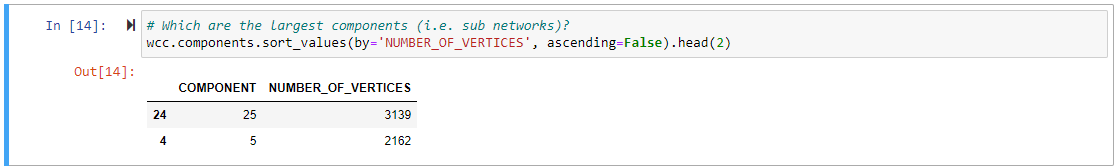
Since components is a Pandas data-frame, we use Pandas capabilities to return only the two largest components - 25 and 5. With wcc.vertices the algorithm provides a data-frame that maps each vertex to the component it belongs to. Let's store the components to SAP HANA and use the subgraph() method of the graph for our visualization. We use the same method to upload the data to SAP HANA we used when we created the graph. The following statement stores the algorithm results to HANA.
hdf_wcc = create_dataframe_from_pandas(

connection_context=cc,

pandas_df=wcc.vertices,

drop_exist_tab=True,

table_name='LM_STORMWATER_WCC',

force=True,

allow_bigint=True,

primary_key='ID')
Sub-Graphs
As we have seen, the components 25 and 5 are the biggest ones in the graph. Let’s put them on a map to gain further insights. The Graph object provides a method to create subgraphs based on filter criteria on vertices or edges.
g_storm_comp1 = g_storm.subgraph(

workspace_name = "LM_STORMWATER_COMP1",

vertices_filter='ID IN (SELECT ID FROM LM_STORMWATER_WCC WHERE COMPONENT = 25)',

force = True

)
This creates a new graph with the name LM_STORMWATER_COMP1 based on a vertex filter. The filter selects only vertices from the components we persisted in the step before and which belong to component 25. In other words, we now have a new graph, i.e. vertices and edges that belong to component 25. We do the same for the vertices of component 5.
g_storm_comp2 = g_storm.subgraph(

workspace_name = "LM_STORMWATER_COMP2",

vertices_filter='ID IN (SELECT ID FROM LM_STORMWATER_WCC WHERE COMPONENT = 5)',

force = True

)
Like before, we use Kepler to visualize the two largest weakly connected components.

Upstream and Downstream Analysis
In this section, we evaluate how one could analyze which sections of our water network could cause a problem reported on a specific access point (i.e. vertex). We look at Neighbors, NeigborsSubgraphs and ShortestPath algorithms.
Get some Information about the Vertex
Let's assume somebody reported a problem with the node WCC_SW002719 (e.g. there is less flow than expected which might indicate a broken pipe somewhere else). We want to analyze that further. First, let's load the vertex itself. We use the same mechanisms we already used before. Since we want to map it later, we materialize the geo-location as a GeoJSON string.

Neighbors
Let's use the Neighbors algorithm to find all neighbors to our reported vertex and display the 5 closest:

If we want to plot the vertices on the map, we need to read the geometries from the database. For that we use the filter() method of the HANA data-frame.
vkc=g_storm_comp2.vertex_key_column

in_list = neighbors.vertices.ID.str.cat(sep="','")

filter = f"{vkc} IN ('{in_list}')"  # Dynamically build the filter condition as SQL WHERE

print(filter)


pdf_storm_comp2_neighbors = g_storm_comp2.vertices_hdf \

.filter(filter) \

.select('ID', ('SHAPE_GEO.ST_TRANSFORM(4326).ST_ASGEOJSON()', 'GJ')).collect()
With that we query and materialize all the geo-locations of all vertices which are 5 hops away from our start vertex. Now we plot the "problem" node and its neighbors.

Upstream and Downstream with NeighborsSubgraph
The image above only shows the vertices reachable within 5 hops from the start vertex. However, when we want to find out what's the root cause of our reported problem, we need to identify all connected vertices. The water network is a directed graph, which means, we're only interested in upstream nodes, because if we see an issue on a node (e.g. less flow than expected), the root cause must be somewhere upstream (i.e. incoming to the node we're looking at). So instead of individual points let's look at subgraphs again.
g_neighbors_upstream = hga.NeighborsSubgraph(graph=g_storm_comp2).execute(

start_vertex=start_vertex_id, direction='INCOMING',

lower_bound=0, upper_bound=10000)
This creates a subgraph starting from a given vertex and only evaluates incoming edges (i.e. upstream in a directed graph). We use the same approach for downstream, i.e. following outgoing edges of the start node.
g_neighbors_downstream = hga.NeighborsSubgraph(graph=g_storm_comp2).execute(

start_vertex=start_vertex_id, direction='OUTGOING',

lower_bound=0, upper_bound=10000)
Like above, g_neighbors_downstream.edges returns only the source and target IDs without the additional information. We've got to load the spatial information of the edges in a separate step again.
ekc = g_storm_comp2.edge_key_column


in_list = g_neighbors_upstream.edges.ID.astype(str).str.cat(sep=',' )

pdf_storm_comp2_neighbors_upstream_edges = g_storm_comp2.edges_hdf \

.filter(f"{ekc} IN ({in_list})") \

.select('ID', ('SHAPE_GEO.ST_TRANSFORM(4326).ST_ASGEOJSON()', 'GJ')).collect()


in_list = g_neighbors_downstream.edges.ID.astype(str).str.cat(sep=',' )

pdf_storm_comp2_neighbors_downstream_edges = g_storm_comp2.edges_hdf \

.filter(f"{ekc} IN ({in_list})") \

.select('ID', ('SHAPE_GEO.ST_TRANSFORM(4326).ST_ASGEOJSON()', 'GJ')).collect()
Looking at the map we understand that we might need to investigate the red, upstream part of the network. The question now is, in which order to check the intakes, to find the one causes problems.

ShortestPathOneToAll
The ShortestPathOneToAll calculates all shortest path distances from one vertex (our reported node), to all the other vertices in the graph.

With direction='INCOMING' we specify that we're only interested in the upstream (i.e. incoming) vertices. weight='LENGTH_M' specifies which column is used to calculate the 'distance'. In our case, we take the length of the pipe segment. If none is specified, the algorithm calculates hop distance. With this information we could investigate our network, assuming that it makes sense to start looking at closer vertices first to find the problem.
Summary
A lot of data science work is done in Python. The hana-ml library provides easy access to SAP HANA, including its spatial and graph capabilities. In this blog post, we explored some of the features introduced with the latest release, hana-ml 2.9.21070902. For demonstration purposes we investigated a stormwater network, but the analysis processes are similar in other domains like transportation, supply, or production chains. In specific, we explained how to
- connect a Jupyter Notebook to SAP HANA
- load data and create a graph in SAP HANA
- visualize the graph using KeplerGL
- analyzing the graph using Strongly Connected Components, SubGraphs, Neighbors, and Shortest Path
The complete script and data is available on github and may serve as a template which you can easily adapt to your domain. To explore the details yourself, just create a free SAP HANA Cloud Trial instance or use an existing SAP HANA Cloud instance.
References
[1] Jupyter Notebook and data on github
[2] SAP HANA Cloud trial
[3] hana-ml on pypi.org
[4] hana-ml documentation
- SAP Managed Tags:
- SAP HANA Cloud,
- SAP HANA Graph,
- SAP HANA multi-model processing,
- SAP HANA Spatial
Labels:
2 Comments
You must be a registered user to add a comment. If you've already registered, sign in. Otherwise, register and sign in.
Labels in this area
-
ABAP CDS Views - CDC (Change Data Capture)
2 -
AI
1 -
Analyze Workload Data
1 -
BTP
1 -
Business and IT Integration
2 -
Business application stu
1 -
Business Technology Platform
1 -
Business Trends
1,658 -
Business Trends
93 -
CAP
1 -
cf
1 -
Cloud Foundry
1 -
Confluent
1 -
Customer COE Basics and Fundamentals
1 -
Customer COE Latest and Greatest
3 -
Customer Data Browser app
1 -
Data Analysis Tool
1 -
data migration
1 -
data transfer
1 -
Datasphere
2 -
Event Information
1,400 -
Event Information
66 -
Expert
1 -
Expert Insights
177 -
Expert Insights
299 -
General
1 -
Google cloud
1 -
Google Next'24
1 -
Kafka
1 -
Life at SAP
780 -
Life at SAP
13 -
Migrate your Data App
1 -
MTA
1 -
Network Performance Analysis
1 -
NodeJS
1 -
PDF
1 -
POC
1 -
Product Updates
4,577 -
Product Updates
344 -
Replication Flow
1 -
RisewithSAP
1 -
SAP BTP
1 -
SAP BTP Cloud Foundry
1 -
SAP Cloud ALM
1 -
SAP Cloud Application Programming Model
1 -
SAP Datasphere
2 -
SAP S4HANA Cloud
1 -
SAP S4HANA Migration Cockpit
1 -
Technology Updates
6,873 -
Technology Updates
423 -
Workload Fluctuations
1
Related Content
- SAP HANA Cloud Vector Engine: Quick FAQ Reference in Technology Blogs by SAP
- Augmenting SAP BTP Use Cases with AI Foundation: A Deep Dive into the Generative AI Hub in Technology Blogs by SAP
- 10+ ways to reshape your SAP landscape with SAP Business Technology Platform – Blog Series in Technology Blogs by SAP
- SAP Business AI : Infuse AI in applications using SAP BTP (with some Use Cases) in Technology Blogs by SAP
- What’s New in SAP HANA Cloud – December 2023 in Technology Blogs by SAP
Top kudoed authors
| User | Count |
|---|---|
| 40 | |
| 25 | |
| 17 | |
| 14 | |
| 8 | |
| 7 | |
| 7 | |
| 7 | |
| 6 | |
| 6 |