
- SAP Community
- Products and Technology
- Technology
- Technology Blogs by SAP
- Anomaly Forecast of Sensor Data in Energy Intensiv...
Technology Blogs by SAP
Learn how to extend and personalize SAP applications. Follow the SAP technology blog for insights into SAP BTP, ABAP, SAP Analytics Cloud, SAP HANA, and more.
Turn on suggestions
Auto-suggest helps you quickly narrow down your search results by suggesting possible matches as you type.
Showing results for
Advisor
Options
- Subscribe to RSS Feed
- Mark as New
- Mark as Read
- Bookmark
- Subscribe
- Printer Friendly Page
- Report Inappropriate Content
04-22-2021
10:26 AM
Introduction
This blog post provides easy reference and sample code for some of the functionality typically required when dealing with Time Series data. For detailed background of some of the real world problems in this area refer to part 1 of this blog post by rafael.pacheco
Anomaly Forecast of Sensor Data in Energy Intensive Industries – Part I: The Machine Learning and Be...
Overall Architecture
Here is a high-level overview of parts of the SAP Business Technology Platform that will be discussed for the anomaly prediction of sensor data
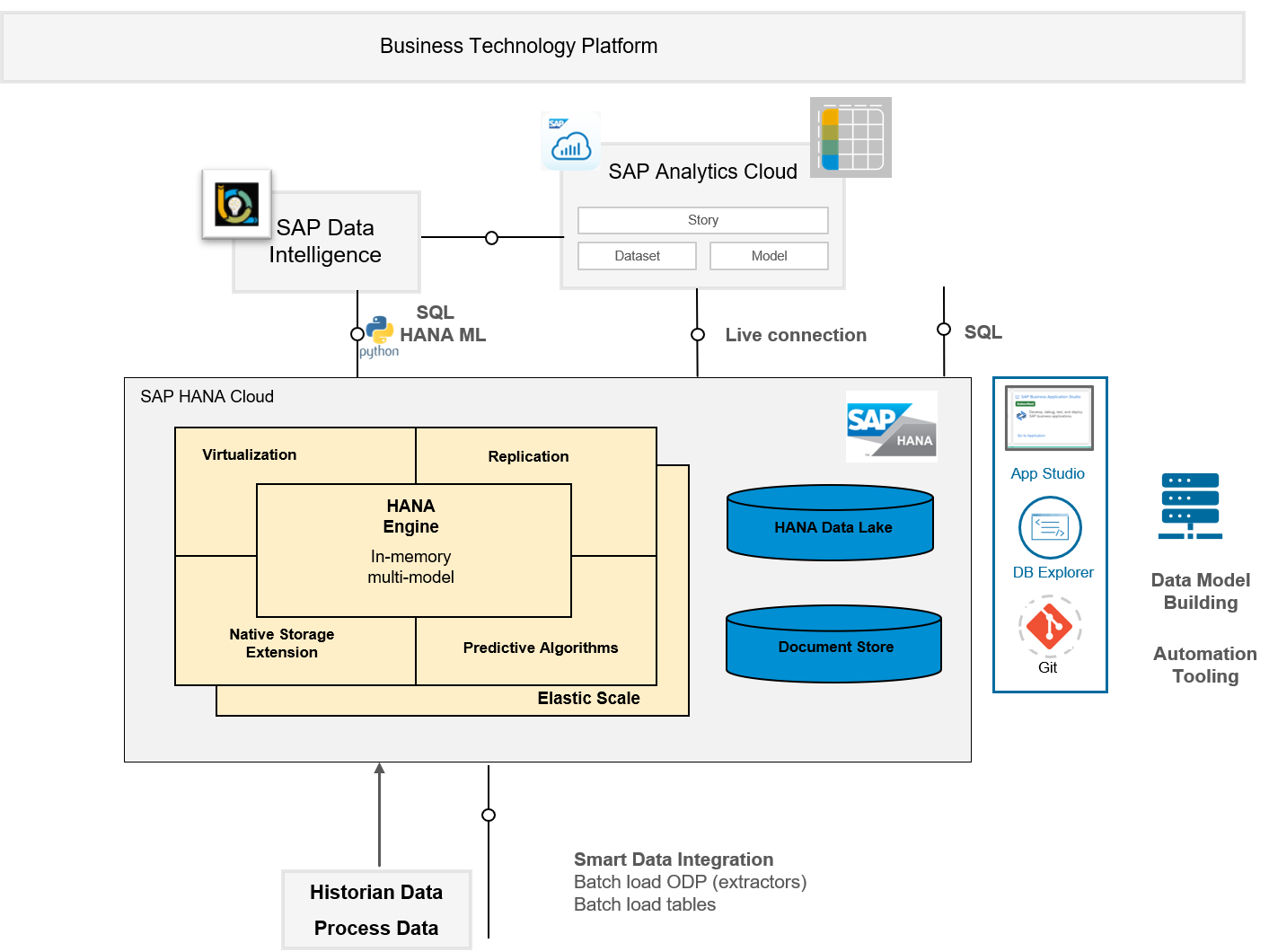
High Level Overview of Technology Components
The blog post will cover the typical ML Model Life cycle in the context of usecase:

ML Model Lifecycle
Dealing with Sensor Data
In today's automated industrial production scenarios there are tens or hundreds of sensor constantly generating new data which could provide vital information on both the current and predicted operational metrics. This data can also be analyzed historically to find root-cause analysis retrospectively. In this blog post we will focus on how to extract information from this data in order to predict anomalies in the near future, on the order of minutes so as corrective action can be taken and the production process can continue with minimal disruption while maintaining quality.
Challenges with Sensor Data
Sensor data from a manufacturing process typically has a few characteristics which need to be dealt with before that data is fit for use in a Machine Learning algorithm. The data needs to be cleaned for duplicates and checked for consistency, which we will not describe here but assume that the available data has been persisted after such checks. The sensor comes in at uneven time intervals across the many sensors as these are not necessarily synchronized as the data is recorded when there is a change in value.
Here I will describe the functionality provided by SAP HANA natively for processing the data. I will use the functionality provided by SAP HANA SQL directly or via SAP HANA Python Client API
The functionality covered here works for both Cloud and On-prem releases for SAP HANA and SAP Data Intelligence.
Turning Sensor Data into Time Series Data
Here is a sample of data coming from 40+ different sensors which has been persisted in SAP HANA database table called HISTORIAN.

To analyze the different signals recorded at uneven time points the first step is to harmonize the data at a defined time interval. The choice of time interval is dependent on the data and underlying frequency it is being generated. SAP HANA Time Series provides easy functionality for data harmonization without having to deal with inherent nuances of time dimension.
For the above case lets say we decide to analyze the data equidistant at a 30 second interval, this can be done with the SERIES_ROUND function
SELECT SERIES_ROUND(DATETIME, 'INTERVAL 30 SECOND') AS TS ,* FROM HISTORIANThis will create equi-spaced data:

Smoothing Sensor Data
The next step it to detect abnormal or anomalous events in the sensor data. However, in many cases it is not desirable to detect all abnormal values from the sensors but only consistently abnormal values to ensure the analysis is not impacted by spikes which could come from data quality issues.
In our example the target signal whose anomalous behaviour we want to analyze is the SIGNAL P_STEAM_SUPPLY provided by TAG38 in the data above. The raw data looks like this:

Lets say we want to smooth the data for a rolling window of 5 minutes and calculate their rolling average
SELECT TS, WEIGHTED_AVG(AVG_PRESSURE) OVER (ORDER BY TS ROWS BETWEEN 10 PRECEDING AND CURRENT ROW) AS MOVING_AVG_5MINUTES FROM

	(SELECT SERIES_ROUND(DATETIME, 'INTERVAL 30 SECOND') AS TS, AVG(VALUE) AS AVG_PRESSURE

        FROM HISTORIAN WHERE SIGNAL = 'P_STEAM_SUPPLY'

        GROUP BY SERIES_ROUND(DATETIME, 'INTERVAL 30 SECOND'))
Pivoting Sensor Data
Now in order to create a predictive model which can predict whether or not the target signal drop below a certain value we would need to pivot the data so we can have the different signals as potential features for the ML Model. In order to do this we can use the pivoting functionality provided by python hana_ml package and detailed in this blog post Pivoting Data with SAP HANA
sql_cmd =

'SELECT * SERIES_ROUND(DATETIME, 'INTERVAL 30 SECOND') AS TS,DATETIME,SIGNAL,TAGNAME,VALUE,UOM ORDER BY TAGNAME'

ts_data = hd.DataFrame(conn, sql_cmd)

print(ts_data.head(5).collect())


ts_pivot = ts_data.pivot_table(index='TS', columns='SIGNAL', values='AVG_VALUE')

ts_pivot.head(5).collect()
The pivoted data will be like below:

ML Model Development
Now that we have the data in the desired format, we can move the step of building a predictive model using native ML capabilities provided by SAP HANA.
The ML capabilities of HANA cover a wide range of algorithms which are available via SQL or Python APIs. For this example we will use the Auto-ML capabilities provided by Automated Predictive Library (APL) fuctionality and in particular the auto-classification model.
Lets say we have data over historic period and collected data prior to the event of pressure drop over a threshold. Together with this data we also collect process data providing information on operating condition metrics for example, number of batches, recipes and completion percentages across different consumption lines. The dataset has labeled whether or not there will be a pressure drop after 5,10,15,20 minutes as described in the results section of the part 1 of this blogpost
Step1: Split the dataset in training & validation dataset

Training Dataset
If the dataset is imbalanced which is likely the case with anomalies we can first upsample with SMOTE using the native HANA ML functionality for this
from hana_ml.algorithms.pal.preprocessing import SMOTE

smote = SMOTE()

new_df = smote.fit_transform(data=df, label = 'TARGET_LEAD_20',minority_class = 1)
This provides a balanced dataset which we can then split into training and hold-out sets
import hana_ml.algorithms.pal.partition as partition


train, test, valid = partition.train_test_val_split(data=df, training_percentage = 0.7, testing_percentage = 0, validation_percentage = 0.3, partition_method='stratified',stratified_column = 'TARGET_LEAD_20')


print("Training Set :", train.count())

print("Validation Set :", valid.count())

print("Fraction of data with in Training DataSet Target 1:", round(train.filter('TARGET_LEAD_20 = 1').count()/train.count()*100,2))

print("Fraction of data with in Validation DataSet Target 1:", round(valid.filter('TARGET_LEAD_20 = 1').count()/valid.count()*100,2))
We do not need to create a test set as the APL library function will do that on its own
Step 2: Train the model
import hana_ml.algorithms.apl as apl

from hana_ml.algorithms.apl.gradient_boosting_classification import GradientBoostingBinaryClassifier


model = apl.gradient_boosting_classification.GradientBoostingBinaryClassifier()

model.fit(train,features = features, label=TARGET_LEAD_20, key='TIMESTAMP_STR')
Step 3:Check Model Quality
model.get_performance_metrics()

##Get feature importance

model.get_feature_importances()['ExactSHAP']


##Check model on hold-out set

score = model.score(valid)

print("Model score:", score)
Step 4: Save the ML Model in HANA
import hana_ml.model_storage

from hana_ml.model_storage import ModelStorage

model_storage = ModelStorage(connection_context=conn)

model.name = 'MY_MODEL_NAME'

model_storage.save_model(model=model, if_exists='replace')
ML Model Deployment
In the current scenario typically we would want to keep updating training data as more anomalies in the data appear which would require frequent training and re-training steps. The automation of the above model training can be achieved via SAP Data Intelligence.
SAP Data Intelligence provides a few different options to create an ML Training Model. It comes with ready to use templates which can help create the training pipeline in matter of minutes.
In the ML Scenario Manager of SAP's Data Intelligence create a pipeline of type HANA ML Training

ML Template

This creates a pipeline which has configurable operators. In our case we configure it for the steps above, for example the table which has the training data, which fields to use as Target, how to split the data between training and test, which ML algorithm to use:

When the pipeline is executed it will save the model as an artifact which is later used for inference on new data. It also generates the accuracy score by default.

The template pipeline provides ready-to-use functionality to create a pipeline which can then be set to run on a scheduled basis.
ML Training Customizations
However, there could be cases where this template is not sufficient. For example, one needs to do some preprocessing or upsampling in our case before we do the training step. In this case you can extend the template with additional operators to process the additional steps. SAP Data Intelligence comes with many in-built operators. Incase these are not sufficient custom operators can be built as described in this Custom Operator blog post
Also for some algorithms like classification it is not sufficient to monitor the accuracy, additionally you would like to track the f1 scores. This can be done via configuring the operator to track additional metrics as described here SAP Data Intelligence Tips & Tricks blog post.
ML Model Consumption
Now that we have a pipeline which creates ML models, we can use the generated model to infer on new data, the whole reason we came down this path so we can predict in advance when the pressure will drop as we get new data.
To enable this again SAP Data Intelligence provides template pipelines which can take a previously generated model and apply on new data. For this we use the HANA ML Inference on Dataset or HANA ML Inference on API Requests, depending on how the new data is available.

This pipeline takes as input the model artifact id which is available from the training step above.
![]()
As with the training you then configure the SAP HANA Connection where the inference should take place. This could be different from where the training was done.
Incase the inference needs to be done independent of SAP HANA then its also possible to use the Java Script version of the ML model as described in the blog post by stojanm MLOps in practice: Applying and updating Machine Learning models in real-time and at scale
As the inference runs in the background, the monitoring of the process can be done via dashboards from SAP Analytics Cloud which provides live connectivity to SAP HANA and monitor the upcoming alerts in real-time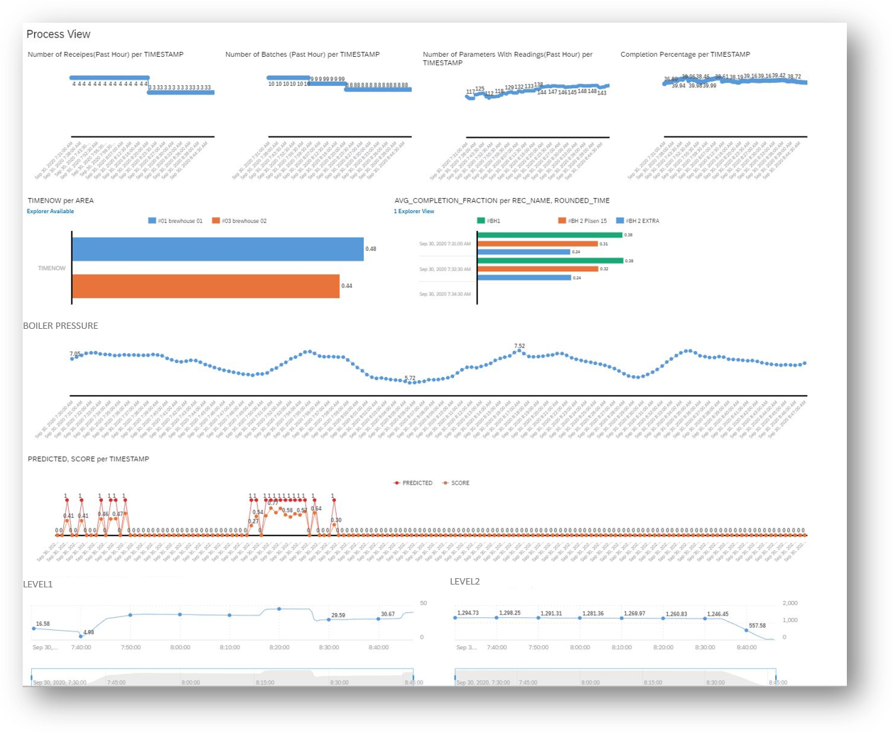
SAP Analytics Cloud Dashboard Monitoring the process
Conclusion
As I come to the end of my end of my blog post, as always I hope my blog posts are of some help when you find yourself dealing with similar problems, which are recurrent not only for ML under Beer Pressure but many ML scenarios under time pressure.
- SAP Managed Tags:
- Machine Learning,
- SAP Data Intelligence,
- SAP HANA
Labels:
4 Comments
You must be a registered user to add a comment. If you've already registered, sign in. Otherwise, register and sign in.
Labels in this area
-
ABAP CDS Views - CDC (Change Data Capture)
2 -
AI
1 -
Analyze Workload Data
1 -
BTP
1 -
Business and IT Integration
2 -
Business application stu
1 -
Business Technology Platform
1 -
Business Trends
1,661 -
Business Trends
87 -
CAP
1 -
cf
1 -
Cloud Foundry
1 -
Confluent
1 -
Customer COE Basics and Fundamentals
1 -
Customer COE Latest and Greatest
3 -
Customer Data Browser app
1 -
Data Analysis Tool
1 -
data migration
1 -
data transfer
1 -
Datasphere
2 -
Event Information
1,400 -
Event Information
64 -
Expert
1 -
Expert Insights
178 -
Expert Insights
273 -
General
1 -
Google cloud
1 -
Google Next'24
1 -
Kafka
1 -
Life at SAP
784 -
Life at SAP
11 -
Migrate your Data App
1 -
MTA
1 -
Network Performance Analysis
1 -
NodeJS
1 -
PDF
1 -
POC
1 -
Product Updates
4,577 -
Product Updates
326 -
Replication Flow
1 -
RisewithSAP
1 -
SAP BTP
1 -
SAP BTP Cloud Foundry
1 -
SAP Cloud ALM
1 -
SAP Cloud Application Programming Model
1 -
SAP Datasphere
2 -
SAP S4HANA Cloud
1 -
SAP S4HANA Migration Cockpit
1 -
Technology Updates
6,886 -
Technology Updates
403 -
Workload Fluctuations
1
Related Content
- Consolidation Extension for SAP Analytics Cloud – Automated Eliminations and Adjustments (part 1) in Technology Blogs by Members
- CAP LLM Plugin – Empowering Developers for rapid Gen AI-CAP App Development in Technology Blogs by SAP
- Embrace the Future: Transform and Standardize Operations with Chatbot in Technology Blogs by Members
- SAP Datasphere - Space, Data Integration, and Data Modeling Best Practices in Technology Blogs by SAP
- Workload Analysis for HANA Platform Series - 1. Define and Understand the Workload Pattern in Technology Blogs by SAP
Top kudoed authors
| User | Count |
|---|---|
| 12 | |
| 10 | |
| 9 | |
| 7 | |
| 7 | |
| 7 | |
| 6 | |
| 6 | |
| 5 | |
| 4 |