
- SAP Community
- Groups
- Interest Groups
- Artificial Intelligence and Machine Learning
- Blogs
- Bayesian Change Point Dectection under Complex Tim...
Artificial Intelligence and Machine Learning Blogs
Explore AI and ML blogs. Discover use cases, advancements, and the transformative potential of AI for businesses. Stay informed of trends and applications.
Turn on suggestions
Auto-suggest helps you quickly narrow down your search results by suggesting possible matches as you type.
Showing results for
former_member73
Discoverer
Options
- Subscribe to RSS Feed
- Mark as New
- Mark as Read
- Bookmark
- Subscribe
- Printer Friendly Page
- Report Inappropriate Content
03-24-2021
7:29 PM
A complex time series in real life usually has many change points inside it. When dealing with such data, simply applying traditional seasonality test to it may not render a convincing decomposition result. In this blog post, we will show how to use Bayesian Change Point Detection in the Python machine learning client for SAP HANA(hana-ml) to detect those change points and decompose the target time series.
In this blog post, you will learn:
Time series may not ideally contain monotonic trend and seasonal waves after decomposition. On the contrary, it may include a great many inner change points in those parts.
As illustrated above, we can see an obvious changing trend and seasonal wave from the time series. Currently, most algorithms are not able to extract them correctly due to the lack of change point analysis. In SAP HANA PAL and hana-ml, we provide BCPD to tackle that.
In this blog post, we will focus on the task of detecting the change points within the varying trend and seasonal components of complex time series.
Bayesian Change Point Detection(BCPD), to some extent, can been seen as an enhanced version of seasonality test in additive mode. Similarly, it decomposes a time series into three components: trend, seasonal and random, but with a remarkable difference that it is capable of detecting change points within both trend and season parts, using a quasi RJ-MCMC method.
Like the additive decomposition in seasonality test, we treat the time series Y(t) as an addition of trend part T and seasonal part S along with random noise:
=T(t,\theta_T)+S(t,\theta_S) +\epsilon(t))
where are the parameters in the trend part, composed of the positions of trend change points and the coefficients
  for each separated segment. Specifically, any trend segment can been written as
%20=%20%5Csum_%7Bi=0%7D%5E%7Btrend%5Ctext%7B%5C_%7Dorder%7D%5Cgamma_i*t%5Ei)
Likewise, are the parameters in the seasonal part, composed of the positions of seasonal change points and the coefficients for each seasonal segment, i.e.
 ) and we may have
and we may have
 = \sum_{l=1}^{harmonic\text{\_}order}[\alpha_l*sin(\frac{2\pi lt}{period})+\beta_l*cos(\frac{2\pi lt}{period})])
One notable thing is that periods in different seasonal segments can vary from one to another, which expands our algorithm to much wider scenarios.
All source code in examples of the following context will use Python machine learning client for SAP HANA Predictive Analsysi Library(PAL).
In this use case, we will focus on detecting the change points in the trend part only,
The mocking data is stored in database in a table with name ‘PAL_MOCKING_BCPD_DATA_1_TBL’, we can use the table() function of ConnectionContext to create a corresponding hana_ml.DataFrame object for it.
The collect() function of hana_ml.DataFrame can help to fetch data from database to the python client and the data is illustrated as follows:
The data is of length 40, then we import the BCPD algorithm from hana-ml and apply it to the mocking dataset:
Again we can use collect() to get the final results from the database. Since we are only interested in the trend part, we can visualize that using the following code:
In this use case, we are to apply BCPD to the data shown in Fig1, in which the trend and season are changing.
Similarly, the data is stored in database in a table with name ‘PAL_MOCKING_BCPD_DATA_2_TBL’ and we need to adjust our parameters for this use case
The trend visualization code is the same as Use case I and the trend plot rendered is:
Further, we use the following code to visualize the seasonal part:
The above plots reveal that BCPD is able to give decent decomposition results on both trend and seasonal parts from the time series.
In this use case, we are going to apply BCPD to real life sensor data to detect potential abrupt change points and to cancel the random term after decomposition for denoising .
Assume the data is stored in a dataframe named sensor_df , we firstly visualize the data using the following code:
In order to obtain a better fit, we are going to use a second-order trend in BCPD for this use case :
After the algorithm finishes, we use the following code to show potential abrupt change points:
Denoised time series can be restored by simply adding the trend and season parts after decomposition:
In the blog post, we introduced a new SAP HANA ML algorithm for detecting change points in the time series with several use cases under Python machine learning client for SAP HANA(hana-ml).
BCPD can be applied to different scenarios: trend test, seasonality test, change points detection, signal noise cancellation, etc.
If you want to learn more about hana-ml and SAP HANA Predictive Analysis Library (PAL), please refer to the following links:
Learning from Labeled Anomalies for Efficient Anomaly Detection using Python Machine Learning Client...
Import multiple excel files into a single SAP HANA table
In this blog post, you will learn:
- Decomposition for complex time series
- Change point detection with hana-ml
Introduction
Time series may not ideally contain monotonic trend and seasonal waves after decomposition. On the contrary, it may include a great many inner change points in those parts.

Fig1
As illustrated above, we can see an obvious changing trend and seasonal wave from the time series. Currently, most algorithms are not able to extract them correctly due to the lack of change point analysis. In SAP HANA PAL and hana-ml, we provide BCPD to tackle that.
In this blog post, we will focus on the task of detecting the change points within the varying trend and seasonal components of complex time series.
Solutions
Bayesian Change Point Detection(BCPD), to some extent, can been seen as an enhanced version of seasonality test in additive mode. Similarly, it decomposes a time series into three components: trend, seasonal and random, but with a remarkable difference that it is capable of detecting change points within both trend and season parts, using a quasi RJ-MCMC method.
Like the additive decomposition in seasonality test, we treat the time series Y(t) as an addition of trend part T and seasonal part S along with random noise:
where
Likewise,
One notable thing is that periods in different seasonal segments can vary from one to another, which expands our algorithm to much wider scenarios.
All source code in examples of the following context will use Python machine learning client for SAP HANA Predictive Analsysi Library(PAL).
Connect to SAP HANA
import hana_ml

from hana_ml import dataframe

cc = dataframe.ConnectionContext(address='xxx.xxx.xxx.xxx', port=30x15, user='XXXXXX', password='XXXXXX')#account details omitted
Use Case I : Detecting Changing Trend
In this use case, we will focus on detecting the change points in the trend part only,
The mocking data is stored in database in a table with name ‘PAL_MOCKING_BCPD_DATA_1_TBL’, we can use the table() function of ConnectionContext to create a corresponding hana_ml.DataFrame object for it.
mocking_df = cc.table('PAL_MOCKING_BCPD_DATA_1_TBL')The collect() function of hana_ml.DataFrame can help to fetch data from database to the python client and the data is illustrated as follows:
plt.plot(mocking_df.collect()["SERIES"])
Fig2
The data is of length 40, then we import the BCPD algorithm from hana-ml and apply it to the mocking dataset:
from hana_ml.algorithms.pal.tsa.changepoint import BCPD

bcpd = BCPD(max_tcp=5, max_scp=0, random_seed=1)

#tcp: location of trend change points

#scp: location of seasonal change points

#period: period of each seasonal segment

#components: decomposition values of the time series

tcp, scp, period, components = bcpd.fit_predict(data=mocking_df)
Again we can use collect() to get the final results from the database. Since we are only interested in the trend part, we can visualize that using the following code:
print(tcp.collect())

plt.plot(mocking_df.collect()["SERIES"], label='data')

plt.plot(components.collect()["TREND"], label='trend')

for cp in list(tcp.collect()["TREND_CP"]):

    plt.axvline(x=cp, color="red", linestyle='dashed')

plt.legend(['original series', 'trend component'])

plt.title("Trend component")

plt.show()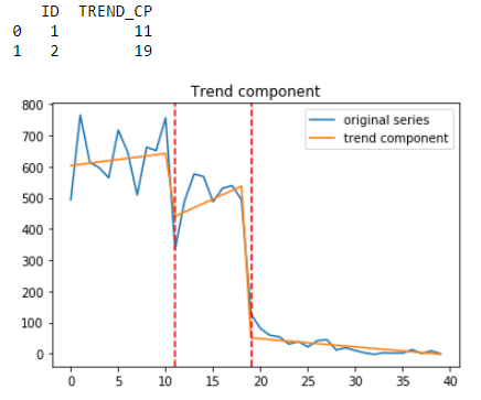
Fig3
Use Case II : Detecting Changing Trend and Season
In this use case, we are to apply BCPD to the data shown in Fig1, in which the trend and season are changing.
Similarly, the data is stored in database in a table with name ‘PAL_MOCKING_BCPD_DATA_2_TBL’ and we need to adjust our parameters for this use case
# detailed introduction of parameters can be found on our user manual page

bcpd = BCPD(max_tcp=5, max_scp=5, max_harmonic_order=1, max_period=10, max_iter=10000, interval_ratio=0.2, random_seed=1)

mocking_df = cc.table('PAL_MOCKING_BCPD_DATA_2_TBL') # data shown in Fig1

tcp, scp, period, components = bcpd.fit_predict(data=mocking_df)
The trend visualization code is the same as Use case I and the trend plot rendered is:

Fig4
Further, we use the following code to visualize the seasonal part:
print(scp.collect())

print(period.collect())

plt.plot(components.collect()["SEASONAL"], label='trend')

for cp in scp.collect()["SEASON_CP"]:

    plt.axvline(x=cp, color="orange", linestyle='dashed')

plt.title("Seasonal component")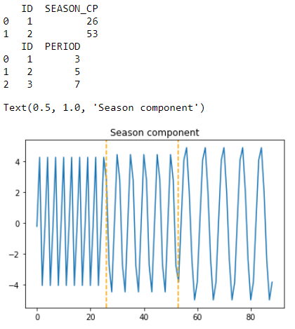
Fig5
The above plots reveal that BCPD is able to give decent decomposition results on both trend and seasonal parts from the time series.
Use Case III : Sensor Data Abrupt Change Detection and Denoising
In this use case, we are going to apply BCPD to real life sensor data to detect potential abrupt change points and to cancel the random term after decomposition for denoising .
Assume the data is stored in a dataframe named sensor_df , we firstly visualize the data using the following code:
figure(num=None, figsize=(10, 3))

plt.plot(sensor_df.collect()["SERIES"])

print(sensor_df.collect())
Fig6
In order to obtain a better fit, we are going to use a second-order trend in BCPD for this use case :
# detailed introduction of parameters can be found on our user manual page

bcpd = BCPD(trend_order=2, max_tcp=10, max_scp=10, max_harmonic_order=10, mmin_period=50, max_period=50, max_iter=15000, interval_ratio=0.01, random_seed=1)

tcp, scp, period, components = bcpd.fit_predict(data=sensor_df)
After the algorithm finishes, we use the following code to show potential abrupt change points:
figure(num=None, figsize=(16, 4), dpi=80, facecolor='w', edgecolor='k')

plt.plot(sensor_df.collect()["SERIES"])

for cp in list(tcp.collect()["TREND_CP"]):

    plt.axvline(x=cp, color="orange", linestyle='dashed')

for cp in scp.collect()["SEASON_CP"]:

    plt.axvline(x=cp, color="orange", linestyle='dashed')

plt.legend(['sensor data', 'potential abrupt change'])

plt.show()
Fig7
Denoised time series can be restored by simply adding the trend and season parts after decomposition:

Fig8
Discussion and Summary
In the blog post, we introduced a new SAP HANA ML algorithm for detecting change points in the time series with several use cases under Python machine learning client for SAP HANA(hana-ml).
BCPD can be applied to different scenarios: trend test, seasonality test, change points detection, signal noise cancellation, etc.
If you want to learn more about hana-ml and SAP HANA Predictive Analysis Library (PAL), please refer to the following links:
Weibull Analysis using Python machine learning client for SAP HANA
Outlier Detection using Statistical Tests in Python Machine Learning Client for SAP HANA
Outlier Detection by Clustering using Python Machine Learning Client for SAP HANA
Outlier Detection with One-class Classification using Python Machine Learning Client for SAP HANA
Learning from Labeled Anomalies for Efficient Anomaly Detection using Python Machine Learning Client...
Additive Model Time-series Analysis using Python Machine Learning Client for SAP HANA
Import multiple excel files into a single SAP HANA table
COPD study, explanation and interpretability with Python machine learning client for SAP HANA
- SAP Managed Tags:
- Machine Learning
You must be a registered user to add a comment. If you've already registered, sign in. Otherwise, register and sign in.
Labels in this area
-
Agents
3 -
AI
5 -
AI Launchpad
2 -
Artificial Intelligence
2 -
Artificial Intelligence (AI)
3 -
Brainstorming
1 -
BTP
1 -
Business AI
2 -
Business Trends
1 -
Cloud Foundry
1 -
Data and Analytics (DA)
1 -
Design and Engineering
1 -
forecasting
1 -
GenAI
1 -
Generative AI
4 -
Generative AI Hub
4 -
Graph
1 -
Language Models
1 -
LlamaIndex
1 -
LLM
2 -
LLMs
2 -
Machine Learning
1 -
Machine learning using SAP HANA
1 -
Mistral AI
1 -
NLP (Natural Language Processing)
1 -
open source
1 -
OpenAI
1 -
Python
2 -
RAG
2 -
Retrieval Augmented Generation
1 -
SAP Build Process Automation
1 -
SAP HANA
1 -
SAP HANA Cloud
1 -
User Experience
1 -
user interface
1 -
Vector Database
3 -
Vector DB
1 -
Vector Similarity
1
Top kudoed authors
| User | Count |
|---|---|
| 5 | |
| 4 | |
| 4 | |
| 1 | |
| 1 |