
- SAP Community
- Products and Technology
- Technology
- Technology Blogs by SAP
- Hands-On Tutorial: Leverage SAP HANA Machine Learn...
Technology Blogs by SAP
Learn how to extend and personalize SAP applications. Follow the SAP technology blog for insights into SAP BTP, ABAP, SAP Analytics Cloud, SAP HANA, and more.
Turn on suggestions
Auto-suggest helps you quickly narrow down your search results by suggesting possible matches as you type.
Showing results for
Product and Topic Expert
Options
- Subscribe to RSS Feed
- Mark as New
- Mark as Read
- Bookmark
- Subscribe
- Printer Friendly Page
- Report Inappropriate Content
02-25-2021
7:19 AM
The hard truth is that many machine learning projects fail to get set into production. It takes time and real effort to move from a machine learning model to a real business application. This is due to many different reasons, for example:
Of course, we can’t save the world with just one Hands-On tutorial, but we can at least try to make the life of a data scientist a little easier. In this blog post we will tackle these challenges by bringing the opensource world and SAP world together. In a nutshell, there will be no movement of training data from SAP HANA Cloud to our Python environment. In the following, we will refer to our SAP HANA Cloud simply as HANA. Of course, you can access the data and sample code under the following GitHub repository. But let us start from the beginning!
As data scientists we feel very comfortable in our RStudio or Python Jupyter Notebooks. We want to stay in our used environment and don’t want to move around in too many different tools. Or even worse, we must copy the code or data from A to B, working on our local laptop with different csv files or other formats. Hence, the great news is that we can directly connect through the R & Python clients with our HANA. Let us look at an example.
In our Python script we first install and import the following library:
The hana_ml library enables us to directly connect to our HANA. To leverage it’s full potential we have to make sure that our user has the following policies assigned:
Set your HANA host, port, user, password and encrypt to true:
Execute the following command to connect to your HANA:
We can hide our login credentials through the Secure User store from the HANA client and don’t have them visible in clear text. In our command prompt we execute the following script:
C:\Program Files\SAP\hdbclient>hdbuserstore -i SET MYHANACLOUD “YOURENDPOINT:PORT” YOURUSERNAME
Then back in our Python script we can use the HANA key to connect:
Now, let us upload a local dataset and push it directly into HANA. Make sure you change the path to your local directory.
Before we bring our local dataset into HANA, we must execute some transformations. We change the columns to upper string and add a unique Product ID to the data. This ID will later be used as a key in our machine learning algorithms, which are directly running in our HANA.
Next, let us create a HANA dataframe and point it to the table with the uploaded data.
Great job! We tackled our first challenge in our machine learning use case. Since, we are now able to directly connect to our HANA from our used environment, let us move to the next task.
Data understanding and preparation take up a lot off time during a machine learning use case. Increasing the data quality can drive every data scientist crazy, due to so many reasons. Hence, let us look at some options we have now through the hana_ml library. Right away our HANA dataframe provides us with different functionalities. Therefore, let us control the data size and if all the variable types are set correctly:
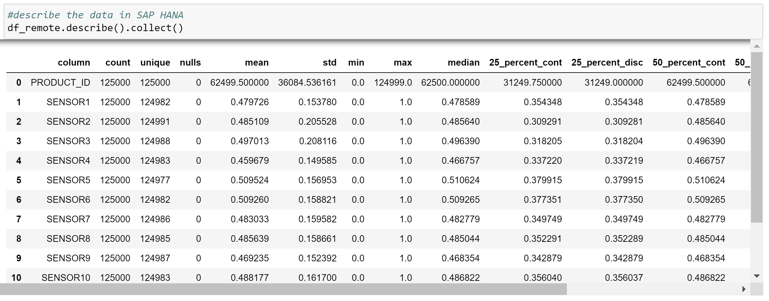
Our data upload was complete but since the variable Quality only contains 0s and 1s, it was falsely set to type integer. The variable is binary and labels all products of bad quality with a 1 and 0 otherwise. Since this is by definition a categorical variable, we transform it to type NVARCHAR with the following command.
To better understand the data, we can derive a description of different statistical attributes or even get a whole data report through the following commands:
If we now find any errors, we have many different functions on hand, staying in our Python environment. For example, we can execute sql commands directly in our Python script or use many more functions available with our HANA dataframe.
At some point we must bring the data and the algorithms together to train our machine learning models. Since our HANA is not only an in-memory database, we don’t have to collect the data into our local environment. Instead we can leverage the native machine learning libraries directly in our HANA. Therefore, let us split the data into a training and testing set through the Predictive Analysis Library (PAL).
Further, let us train and optimize a random forest algorithm to classify the quality of a product. First, we set the numbers of trees very high, to see where the Out of Bag error converges. After optimizing the numbers of trees, we will take a closer look at the variables considered at each split.
Now, we can apply our trained model on the testing set.
For each observation we can see the predicted class and of course the confidence of our random forest model. In addition, we can compute the confusion matrix or a have a look at the variable importance.
The idea is to keep the heavy lifting in our HANA and only collect small sets to for example evaluate our random forest model. Therefore, we can collect the OOB error and use opensource libraries to visualize the results:
Our trained model converges after around 700 trees. Hence, let us set the parameter to 801 trees to leave a little buffer. Further, let us optimize the number of variables considered at each split by iterating through each possible value.

After 2 variables considered at each split the error increases and we must be careful not to overfit the data. Therefore, let us train our optimal random forest model.
Congratulation, you created your first machine learning model directly in HANA. Now, let’s move to our last pain point.
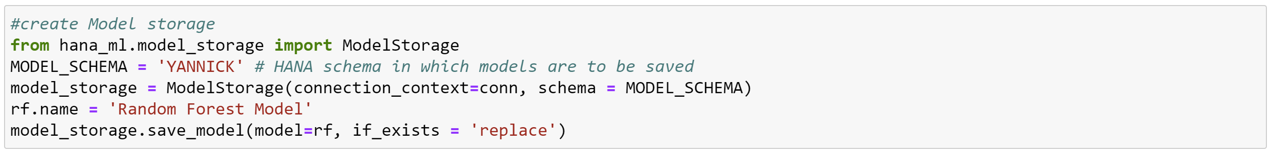
After the evaluation of our machine learning model a last very crucial step is still missing. We must deploy our model into the IT landscape and make our new insights accessible to the business, such that they can incorporate this information into their decision making. Our huge advantage is now that our machine learning model already resides in HANA. We can create a Model Storage where we can save our trained model and load it again for consumption. Hence, please execute the following script:
Let’s view the saved model in our model storage.
Of course, we can now save additional tables created based on our model and consume them in different frontend tools like the SAP Analytics Cloud. For example, have a look at the following blogs:
In addition, if you like to try the Automated Predictive Library (APL) or are a big R fan, try out the following Hands-On tutorials:
I hope this blog post helped you to get started with your own SAP Machine Learning use cases. I encourage you to try it yourself and bring more machine learning into production.
I want to thank andreas.forster, christoph.morgen and sarah.detzler for their support while writing this Hands-On tutorial.
Cheers!
Yannick Schaper
- Limited data access
- Poor data quality
- Small computing power
- No version control
Of course, we can’t save the world with just one Hands-On tutorial, but we can at least try to make the life of a data scientist a little easier. In this blog post we will tackle these challenges by bringing the opensource world and SAP world together. In a nutshell, there will be no movement of training data from SAP HANA Cloud to our Python environment. In the following, we will refer to our SAP HANA Cloud simply as HANA. Of course, you can access the data and sample code under the following GitHub repository. But let us start from the beginning!
- How can we directly access the data in our HANA?
As data scientists we feel very comfortable in our RStudio or Python Jupyter Notebooks. We want to stay in our used environment and don’t want to move around in too many different tools. Or even worse, we must copy the code or data from A to B, working on our local laptop with different csv files or other formats. Hence, the great news is that we can directly connect through the R & Python clients with our HANA. Let us look at an example.
In our Python script we first install and import the following library:


The hana_ml library enables us to directly connect to our HANA. To leverage it’s full potential we have to make sure that our user has the following policies assigned:
- AFL__SYS_AFL_AFLPAL_EXECUTE_WITH_GRANT_OPTION
- AFL__SYS_AFL_APL_AREA_EXECUTE
- AFLPM_CREATOR_ERASER_EXECUTE
Set your HANA host, port, user, password and encrypt to true:

Execute the following command to connect to your HANA:

We can hide our login credentials through the Secure User store from the HANA client and don’t have them visible in clear text. In our command prompt we execute the following script:
C:\Program Files\SAP\hdbclient>hdbuserstore -i SET MYHANACLOUD “YOURENDPOINT:PORT” YOURUSERNAME

Then back in our Python script we can use the HANA key to connect:

Now, let us upload a local dataset and push it directly into HANA. Make sure you change the path to your local directory.

Before we bring our local dataset into HANA, we must execute some transformations. We change the columns to upper string and add a unique Product ID to the data. This ID will later be used as a key in our machine learning algorithms, which are directly running in our HANA.

Next, let us create a HANA dataframe and point it to the table with the uploaded data.

Great job! We tackled our first challenge in our machine learning use case. Since, we are now able to directly connect to our HANA from our used environment, let us move to the next task.
- How can we explore our data and react to data quality issues early?
Data understanding and preparation take up a lot off time during a machine learning use case. Increasing the data quality can drive every data scientist crazy, due to so many reasons. Hence, let us look at some options we have now through the hana_ml library. Right away our HANA dataframe provides us with different functionalities. Therefore, let us control the data size and if all the variable types are set correctly:

Our data upload was complete but since the variable Quality only contains 0s and 1s, it was falsely set to type integer. The variable is binary and labels all products of bad quality with a 1 and 0 otherwise. Since this is by definition a categorical variable, we transform it to type NVARCHAR with the following command.

To better understand the data, we can derive a description of different statistical attributes or even get a whole data report through the following commands:


If we now find any errors, we have many different functions on hand, staying in our Python environment. For example, we can execute sql commands directly in our Python script or use many more functions available with our HANA dataframe.
- How can we leverage the computing power of our HANA in our machine learning use case?
At some point we must bring the data and the algorithms together to train our machine learning models. Since our HANA is not only an in-memory database, we don’t have to collect the data into our local environment. Instead we can leverage the native machine learning libraries directly in our HANA. Therefore, let us split the data into a training and testing set through the Predictive Analysis Library (PAL).


Further, let us train and optimize a random forest algorithm to classify the quality of a product. First, we set the numbers of trees very high, to see where the Out of Bag error converges. After optimizing the numbers of trees, we will take a closer look at the variables considered at each split.

Now, we can apply our trained model on the testing set.

For each observation we can see the predicted class and of course the confidence of our random forest model. In addition, we can compute the confusion matrix or a have a look at the variable importance.


The idea is to keep the heavy lifting in our HANA and only collect small sets to for example evaluate our random forest model. Therefore, we can collect the OOB error and use opensource libraries to visualize the results:

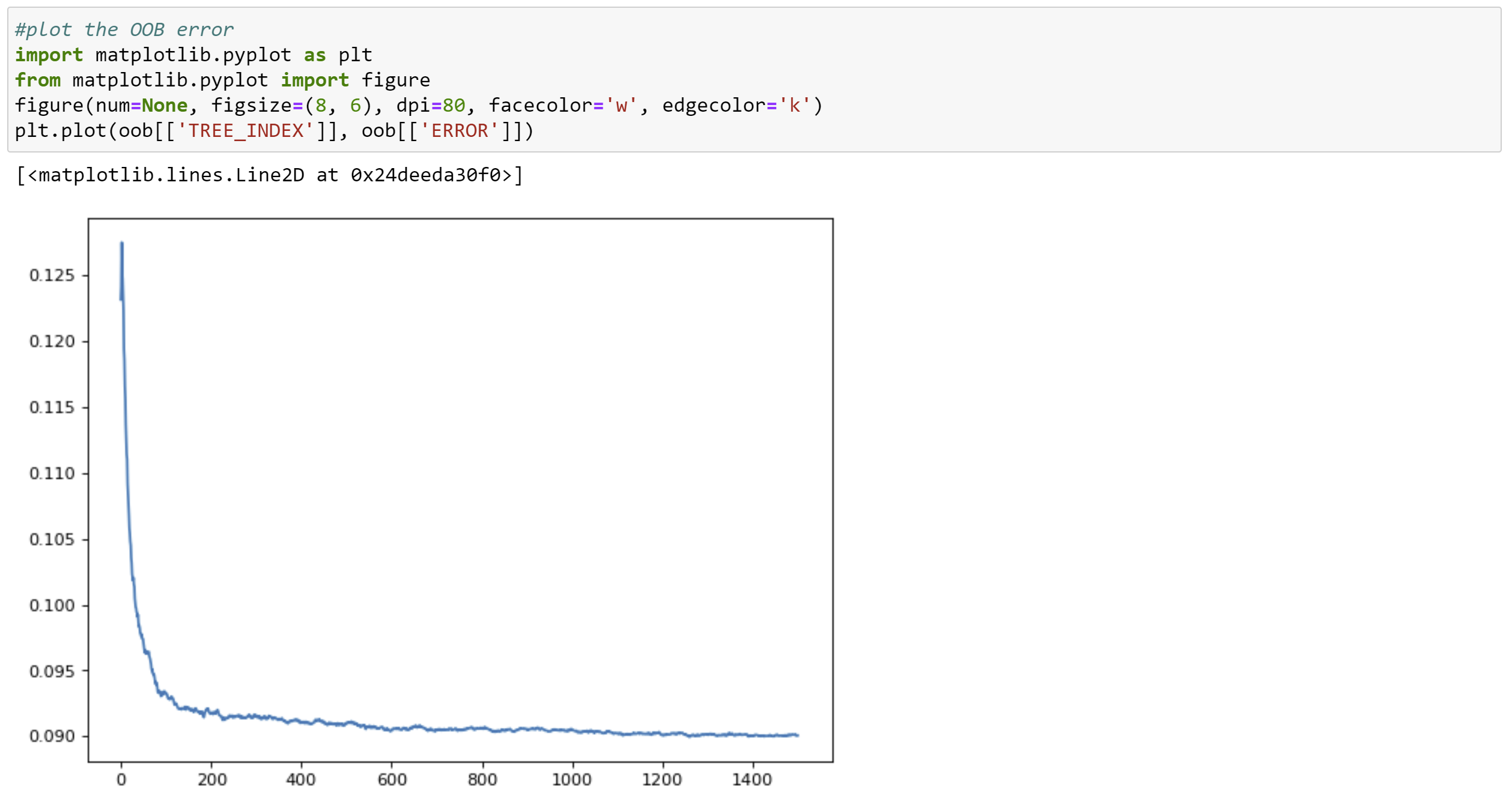
Our trained model converges after around 700 trees. Hence, let us set the parameter to 801 trees to leave a little buffer. Further, let us optimize the number of variables considered at each split by iterating through each possible value.
Let’s plot the result:

After 2 variables considered at each split the error increases and we must be careful not to overfit the data. Therefore, let us train our optimal random forest model.

Congratulation, you created your first machine learning model directly in HANA. Now, let’s move to our last pain point.
- How can we save and create different versions of our results?
After the evaluation of our machine learning model a last very crucial step is still missing. We must deploy our model into the IT landscape and make our new insights accessible to the business, such that they can incorporate this information into their decision making. Our huge advantage is now that our machine learning model already resides in HANA. We can create a Model Storage where we can save our trained model and load it again for consumption. Hence, please execute the following script:
Let’s view the saved model in our model storage.

Of course, we can now save additional tables created based on our model and consume them in different frontend tools like the SAP Analytics Cloud. For example, have a look at the following blogs:
- Story design, formatting, and aesthetics
- SAP Analytics Cloud Learning
- Hands-On Tutorial SAP Analytics Cloud, R Visualization
In addition, if you like to try the Automated Predictive Library (APL) or are a big R fan, try out the following Hands-On tutorials:
- Hands-On Tutorial: Automated Predictive (APL) in SAP HANA Cloud
- Hands-On Tutorial: Leverage SAP HANA embedded Machine Learning through an R Shiny App
- Hands-On Tutorial: Becoming the Chief Data Cook with RStudio and SAP HANA
I hope this blog post helped you to get started with your own SAP Machine Learning use cases. I encourage you to try it yourself and bring more machine learning into production.
I want to thank andreas.forster, christoph.morgen and sarah.detzler for their support while writing this Hands-On tutorial.
Cheers!
Yannick Schaper
- SAP Managed Tags:
- Machine Learning,
- SAP HANA Cloud,
- Data and Analytics,
- Python,
- SAP HANA,
- Big Data
Labels:
7 Comments
You must be a registered user to add a comment. If you've already registered, sign in. Otherwise, register and sign in.
Labels in this area
-
ABAP CDS Views - CDC (Change Data Capture)
2 -
AI
1 -
Analyze Workload Data
1 -
BTP
1 -
Business and IT Integration
2 -
Business application stu
1 -
Business Technology Platform
1 -
Business Trends
1,658 -
Business Trends
91 -
CAP
1 -
cf
1 -
Cloud Foundry
1 -
Confluent
1 -
Customer COE Basics and Fundamentals
1 -
Customer COE Latest and Greatest
3 -
Customer Data Browser app
1 -
Data Analysis Tool
1 -
data migration
1 -
data transfer
1 -
Datasphere
2 -
Event Information
1,400 -
Event Information
66 -
Expert
1 -
Expert Insights
177 -
Expert Insights
293 -
General
1 -
Google cloud
1 -
Google Next'24
1 -
Kafka
1 -
Life at SAP
780 -
Life at SAP
13 -
Migrate your Data App
1 -
MTA
1 -
Network Performance Analysis
1 -
NodeJS
1 -
PDF
1 -
POC
1 -
Product Updates
4,577 -
Product Updates
340 -
Replication Flow
1 -
RisewithSAP
1 -
SAP BTP
1 -
SAP BTP Cloud Foundry
1 -
SAP Cloud ALM
1 -
SAP Cloud Application Programming Model
1 -
SAP Datasphere
2 -
SAP S4HANA Cloud
1 -
SAP S4HANA Migration Cockpit
1 -
Technology Updates
6,873 -
Technology Updates
417 -
Workload Fluctuations
1
Related Content
- SAP HANA Cloud's Vector Engine vs. HANA on-premise in Technology Blogs by Members
- ABAP Cloud Developer Trial 2022 Available Now in Technology Blogs by SAP
- New Machine Learning features in SAP HANA Cloud in Technology Blogs by SAP
- SAP HANA Cloud Vector Engine: Quick FAQ Reference in Technology Blogs by SAP
- 10+ ways to reshape your SAP landscape with SAP Business Technology Platform – Blog 4 in Technology Blogs by SAP
Top kudoed authors
| User | Count |
|---|---|
| 34 | |
| 25 | |
| 13 | |
| 7 | |
| 7 | |
| 6 | |
| 6 | |
| 6 | |
| 5 | |
| 4 |