
- SAP Community
- Products and Technology
- Technology
- Technology Blogs by SAP
- Multi-model in hana_ml 2.6 for Python (part 06): T...
Technology Blogs by SAP
Learn how to extend and personalize SAP applications. Follow the SAP technology blog for insights into SAP BTP, ABAP, SAP Analytics Cloud, SAP HANA, and more.
Turn on suggestions
Auto-suggest helps you quickly narrow down your search results by suggesting possible matches as you type.
Showing results for
Developer Advocate
Options
- Subscribe to RSS Feed
- Mark as New
- Mark as Read
- Bookmark
- Subscribe
- Printer Friendly Page
- Report Inappropriate Content
12-01-2020
2:07 PM
In the previous posts, we did the exploration and visualization of spatial and graph data in HANA dataframes. Now let's' use an example tying it all together.
For that, we will use graphs to calculate the shortest paths and use geospatial to plot these paths on maps.
… I am going to create a new notebook
Then import usual modules and connect to SAP HANA instance (SAP HANA Cloud trial instance in my case).
Nothing new so far. Almost. It is just that we created something I should have done already in an earlier post: reusable notebook. It just escaped from my notes... till now ?
We now create another new notebook
Let's include some other known packages we will use later for plotting geospatial data.
Let's recreate the HANA Graph in Python from the graph workspace we have created in the previous post.
Let's read our original tables to add a calculated column to edges. This column will store geospatial string with the line connecting two ports.
You can see the use of the SAP HANA SQL
Now, this dataframe contains the column
The original
As you can see I used 5280 feet to calculate the mile. That's because SAP HANA's table
A month ago rawatu published a post Find Your Path -- With SAP HANA Graph. You can read there in more detail about the complexity of shortest path calculations and about SAP HANA impressive performance processing those.
SAP HANA's shortest path is available as a
You can plug your own start and end airports, obviously.
The method calculates the shortest path as the path with the smallest number of intermediate nodes if a weight property is not provided.
To be able to show these on the plot we need to create Geopandas dataframes
Now we can use these Geopandas dataframes to plot the calculated path in the way similar to used in the post Multi-model in hana_ml 2.6 for Python: Geospatial visualization!
Please note, that because there are multiple paths with 3 intermediate nodes the algorithm can return different results, like below.
Now let's do the same, but searching for the shortest total distance using the property
Now, similarly to the previous step, we just need to create Geopandas dataframes for nodes and edges...
...and to visualize them.
Thank you for following this series, and I am looking forward to (virtually) seeing you at SAP TechEd 2020 next week!
But before I hit publish, I'd like to thank lynn.scheinman for his work that was a foundation and an inspiration for this series!
Stay healthy ❤️ everyone,
-Vitaliy (aka @Sygyzmundovych)
For that, we will use graphs to calculate the shortest paths and use geospatial to plot these paths on maps.
One more time…
… I am going to create a new notebook
00 Logon.ipynb in JupyterLab.Then import usual modules and connect to SAP HANA instance (SAP HANA Cloud trial instance in my case).
import pandas as pd

from hana_ml import dataframe as dfhhana_cloud_endpoint="<uuid>.hana.trial-eu10.hanacloud.ondemand.com:443"hana_cloud_host, hana_cloud_port=hana_cloud_endpoint.split(":")
cchc=dfh.ConnectionContext(port=hana_cloud_port,
address=hana_cloud_host,
user='HANAML',
password='Super$ecr3t!',
encrypt=True
)Nothing new so far. Almost. It is just that we created something I should have done already in an earlier post: reusable notebook. It just escaped from my notes... till now ?
We now create another new notebook
05 Multimodel.ipynb where we include the previous one as the first step.%run "./00 Logon.ipynb"cchc.connection.isconnected()Let's include some other known packages we will use later for plotting geospatial data.
import geopandas

import contextily as ctx
Create HANA Graph in Python from an existing graph workspace
Let's recreate the HANA Graph in Python from the graph workspace we have created in the previous post.
import hana_ml.graph.hana_graphhana_ml.graph.hana_graph.discover_graph_workspaces(cchc)hgws_airroutes=(
hana_ml.graph.hana_graph
.create_hana_graph_from_existing_workspace(
cchc,
workspace_name='AIRROUTES_DFH')
)Create HANA DataFrame in Python with geospatial strings for connections
Let's read our original tables to add a calculated column to edges. This column will store geospatial string with the line connecting two ports.
dfh_ports=cchc.table("PORTS", geo_cols={"POINT_LON_LAT_GEO":"4326"})

dfh_routes=cchc.table("ROUTES")
dfh_routes_strings=cchc.sql(
dfh_routes.alias('E')
.join(dfh_ports.alias('F'),'E."FROM"=F."ID"', select=['E.*',('POINT_LON_LAT_GEO','POINT_FROM')])
.alias('E2')
.join(dfh_ports.alias('T'),'E2."TO"=T."ID"',
select=[('E2.ID','ID'), 'FROM', 'TO', 'DIST',
('ST_MakeLine("POINT_FROM", "POINT_LON_LAT_GEO")', 'LINE')]
).select_statement, geo_cols={'LINE': 4326}
)
dfh_routes_strings.head(3).collect()You can see the use of the SAP HANA SQL
ST_MakeLine() method to create a string connecting two ports. To make it possible we join the edges table with two instances or port tables to read a location of FROM and TO nodes.
Now, this dataframe contains the column
DIST -- the distance loaded from the source CSV file. We just do not know in what unit this distance was measured. Let's use SAP HANA capabilities to calculate lengths of generated spatial lines in kilometers and in miles.dfh_routes_strings.select(
"*",
('ROUND("LINE".ST_Length(\'foot\')/5280)', "CONV_M"),
('ROUND("LINE".ST_Length(\'kilometer\'))', "CONV_KM")
).head(3).collect()
The original
DIST must be in miles as it is not exactly, but very closely matches the distance converted to miles by SAP HANA.As you can see I used 5280 feet to calculate the mile. That's because SAP HANA's table
ST_UNITS_OF_MEASURE contains predefined foot unit, but not mile.cchc.table("ST_UNITS_OF_MEASURE", schema="PUBLIC").collect()
Calculate and visualize the shortest path
A month ago rawatu published a post Find Your Path -- With SAP HANA Graph. You can read there in more detail about the complexity of shortest path calculations and about SAP HANA impressive performance processing those.
SAP HANA's shortest path is available as a
shortest_path() method, which I am going to use to calculate the shortest path from WRO (Wrocław, Poland) to GKA (Goroka, Papua New Guinea) on the other side of the globe.You can plug your own start and end airports, obviously.
path_wro_to_gka_hops=hgws_airroutes.shortest_path(

    source=str(hgws_airroutes.vertices_hdf.filter("CODE='WRO'").select('ID').collect().values[0][0]),

    target=str(hgws_airroutes.vertices_hdf.filter("CODE='GKA'").select('ID').collect().values[0][0]),

    direction='OUTGOING'

)


print("Number of connectons: {}".format(int(path_wro_to_gka_hops.weight())))

display(path_wro_to_gka_hops.edges().set_index('EDGE_ORDER'))

display(path_wro_to_gka_hops.vertices().set_index('VERTEX_ORDER'))
The method calculates the shortest path as the path with the smallest number of intermediate nodes if a weight property is not provided.
To be able to show these on the plot we need to create Geopandas dataframes
dfg_ for the selected nodes and for the spatial aggregation of connecting lines using ST_CollectAggr().dfg_shortest_path_hops = geopandas.GeoDataFrame(
dfh_ports
.filter('ID IN ('+path_wro_to_gka_hops.vertices().ID.astype(str).str.cat(sep=',')+')')
.select("ID", "CODE", "CITY", "POINT_LON_LAT_GEO").collect(),
geometry='POINT_LON_LAT_GEO', crs="EPSG:4326"
)dfg_shortest_path_string = geopandas.GeoDataFrame(
cchc.sql(
dfh_routes_strings
.filter('ID IN ('+path_wro_to_gka_hops.edges().ID.astype(str).str.cat(sep=',')+')')
.agg([('ST_CollectAggr', 'LINE', 'LINE_PATH')])
.select_statement,
geo_cols={'LINE_PATH':4326}).collect(),
geometry='LINE_PATH', crs="EPSG:4326"
)
Now we can use these Geopandas dataframes to plot the calculated path in the way similar to used in the post Multi-model in hana_ml 2.6 for Python: Geospatial visualization!
fig_shortest_path=dfg_shortest_path_hops.to_crs(epsg=3857).plot(

    figsize=(20, 15), zorder=3,

    alpha=1, color='w', edgecolor='r', markersize=300

)

fig_shortest_path.set_axis_off()


dfg_shortest_path_hops.to_crs(epsg=3857).apply(

    lambda port: fig_shortest_path.annotate(port.CITY,

                                            xy=port.POINT_LON_LAT_GEO.coords[0],

                                            xytext=(-10, 15),

                                            textcoords="offset points",

                                            fontsize="x-large",

                                            color="b"

                                           ), axis=1

)


dfg_shortest_path_string.to_crs(epsg=3857).plot(ax=fig_shortest_path, alpha=1, edgecolor='r', zorder=1)


ctx.add_basemap(ax=fig_shortest_path, source=ctx.providers.OpenStreetMap.Mapnik)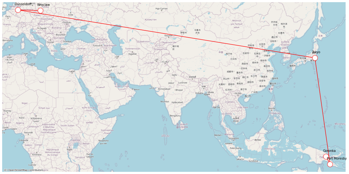
Please note, that because there are multiple paths with 3 intermediate nodes the algorithm can return different results, like below.

...with the shortest distance
Now let's do the same, but searching for the shortest total distance using the property
weight to supply the value of a column DIST.path_wro_to_gka_dist=hgws_airroutes.shortest_path(
source=str(hgws_airroutes.vertices_hdf.filter("CODE='WRO'").select('ID').collect().values[0][0]),
target=str(hgws_airroutes.vertices_hdf.filter("CODE='GKA'").select('ID').collect().values[0][0]),
direction='OUTGOING',
weight='DIST'
)
print("Total distance: {}".format(int(path_wro_to_gka_dist.weight())))
# display(path_wro_to_gka_dist.edges().set_index('EDGE_ORDER'))
# display(path_wro_to_gka_dist.vertices().set_index('VERTEX_ORDER'))
Now, similarly to the previous step, we just need to create Geopandas dataframes for nodes and edges...
dfg_shortest_path_dist_hops = geopandas.GeoDataFrame(

    dfh_ports

    .filter('ID IN ('+path_wro_to_gka_dist.vertices().ID.astype(str).str.cat(sep=',')+')')

    .select("ID", "CODE", "CITY", "POINT_LON_LAT_GEO").collect(),

    geometry='POINT_LON_LAT_GEO', crs="EPSG:4326"

)


dfg_shortest_path_dist_string = geopandas.GeoDataFrame(

cchc.sql(dfh_routes_strings

         .filter('ID IN ('+path_wro_to_gka_dist.edges().ID.astype(str).str.cat(sep=',')+')')

         .agg([('ST_UnionAggr', 'LINE', 'LINE_PATH')])

         .select_statement,

        geo_cols={'LINE_PATH':4326}).collect(), geometry='LINE_PATH', crs="EPSG:4326")
...and to visualize them.
fig_shortest_path_dist=dfg_shortest_path_dist_hops.to_crs(epsg=3857).plot(

    figsize=(20, 15), zorder=3,

    alpha=1, color='w', edgecolor='r', markersize=300

)

fig_shortest_path_dist.set_axis_off()


dfg_shortest_path_dist_hops.to_crs(epsg=3857).apply(

    lambda port: fig_shortest_path_dist.annotate(port.CITY,

                                            xy=port.POINT_LON_LAT_GEO.coords[0],

                                            xytext=(-10, 15), textcoords="offset points",

                                            fontsize="x-large", color="b"

                                           ), axis=1

)


dfg_shortest_path_dist_string.to_crs(epsg=3857).plot(ax=fig_shortest_path_dist, alpha=1, edgecolor='r', zorder=1)


ctx.add_basemap(ax=fig_shortest_path_dist, source=ctx.providers.OpenStreetMap.Mapnik)
And that's it!
Thank you for following this series, and I am looking forward to (virtually) seeing you at SAP TechEd 2020 next week!
But before I hit publish, I'd like to thank lynn.scheinman for his work that was a foundation and an inspiration for this series!
Stay healthy ❤️ everyone,
-Vitaliy (aka @Sygyzmundovych)
- SAP Managed Tags:
- SAP HANA Cloud,
- Python,
- SQL,
- SAP HANA,
- SAP HANA Graph,
- SAP HANA multi-model processing,
- SAP HANA Spatial
Labels:
2 Comments
You must be a registered user to add a comment. If you've already registered, sign in. Otherwise, register and sign in.
Labels in this area
-
ABAP CDS Views - CDC (Change Data Capture)
2 -
AI
1 -
Analyze Workload Data
1 -
BTP
1 -
Business and IT Integration
2 -
Business application stu
1 -
Business Technology Platform
1 -
Business Trends
1,661 -
Business Trends
87 -
CAP
1 -
cf
1 -
Cloud Foundry
1 -
Confluent
1 -
Customer COE Basics and Fundamentals
1 -
Customer COE Latest and Greatest
3 -
Customer Data Browser app
1 -
Data Analysis Tool
1 -
data migration
1 -
data transfer
1 -
Datasphere
2 -
Event Information
1,400 -
Event Information
64 -
Expert
1 -
Expert Insights
178 -
Expert Insights
273 -
General
1 -
Google cloud
1 -
Google Next'24
1 -
Kafka
1 -
Life at SAP
784 -
Life at SAP
11 -
Migrate your Data App
1 -
MTA
1 -
Network Performance Analysis
1 -
NodeJS
1 -
PDF
1 -
POC
1 -
Product Updates
4,577 -
Product Updates
326 -
Replication Flow
1 -
RisewithSAP
1 -
SAP BTP
1 -
SAP BTP Cloud Foundry
1 -
SAP Cloud ALM
1 -
SAP Cloud Application Programming Model
1 -
SAP Datasphere
2 -
SAP S4HANA Cloud
1 -
SAP S4HANA Migration Cockpit
1 -
Technology Updates
6,886 -
Technology Updates
403 -
Workload Fluctuations
1
Related Content
- Forecast Local Explanation with Automated Predictive (APL) in Technology Blogs by SAP
- Enhancing S/4HANA with SAP HANA Cloud Vector Store and GenAI in Technology Blogs by SAP
- Define and insert data into temporary table using python hana_ml in Technology Blogs by SAP
- Consume Machine Learning API in SAPUI5, SAP Build, SAP ABAP Cloud and SAP Fiori IOS SDK in Technology Blogs by Members
- SAP hana_ml ARIMAX with SAP AI Core in Technology Q&A
Top kudoed authors
| User | Count |
|---|---|
| 12 | |
| 10 | |
| 9 | |
| 7 | |
| 7 | |
| 7 | |
| 6 | |
| 6 | |
| 5 | |
| 4 |