
- SAP Community
- Products and Technology
- Technology
- Technology Blogs by SAP
- Multi-model in hana_ml 2.6 for Python (part 03): S...
Technology Blogs by SAP
Learn how to extend and personalize SAP applications. Follow the SAP technology blog for insights into SAP BTP, ABAP, SAP Analytics Cloud, SAP HANA, and more.
Turn on suggestions
Auto-suggest helps you quickly narrow down your search results by suggesting possible matches as you type.
Showing results for
Developer Advocate
Options
- Subscribe to RSS Feed
- Mark as New
- Mark as Read
- Bookmark
- Subscribe
- Printer Friendly Page
- Report Inappropriate Content
11-17-2020
9:29 PM
In the previous post, we looked at the regular data exploration using HANA dataframes. But the objective of this series is to explain the new multi-model functionality of
With
If spatial data with SAP HANA is new to you, I would suggest going through introductory tutorials first:
...let me move back to JupyterLab and create a new notebook
Because this is the new notebook, we will need to load the required Python modules and connect to the SAP HANA instance first.
Please note, that this time I am not using
Let try to query the location of the nearest airport. It will require your rough GPS location's latitude and longitude assigned to two variables
You can provide yours manually there, or we can go a bit geekier and query the location from the same
Let's
In your case, they should be different. And if you are on the VPN, then it might not even be your location at all. Adjust the location manually, if required ?
With these two variables
With this line of code we:
You can verify the generated
As we discussed already, the SQL in a HANA DataFrame is executed only when specific methods, like
So, the nearest airport is
Well, the spatial data is stored in a binary format. To be able to read it properly several methods in
Now the airport's location is represented using the Well-Known Text (or WKT) value
"Isn't it possible to visualize spatial data now that we are using Python and Jupyter?" ask you. Absolutely! And we will get to that, but first, let us finish with the use of
The next question would be what if you want to use HANA DataFrame methods to build the query, not embedded SQL, yet still, return the geospatial columns in the right format? This is where the trick, which I shared as a riddle in the first post, should help -- embedding dfh's
Last note here: check two different ways I used
So far we had to calculate airport spatial points (locations) from
Let's do this now, but it means we need to repeat the step of reading and wrangling data from a CSV file using a Pandas dataframe
And once again we are creating (or rather re-creating SAP HANA table
This time a table in the database was created with the new
Now we can use this column to simplify the previous exploration of data, like finding the nearest airport!
Another great improvement in
We will use an old, but still very popular World Borders shapefile from the Thematic Mapping.
I am going to create a subfolder
Let's use the new
and query the table to check your country, like
As the last example let me show the HANA DataFrame's query joining two tables using the spatial predicate
How many airports are in Poland?
PS. And yes, I know there is a column
...in
Can you modify queries, using the distance unit other than the default meter? Two hints:
As promised, we will focus on the visualization of the geospatial results in the next episode.
And stay healthy ❤️
-Vitaliy (aka @Sygyzmundovych)
PS. And if you read this on November 18th, then Happy GIS Day!
hana_ml 2.6, which I used as well in my demo in SAP TechEd’s DAT108 session.With
hana_ml 2.6 release several HANA DataFrame methods have been extended to support the processing of (geo-)spatial columns. And what is the better time to discuss this if not during Geography Awareness Week?If spatial data with SAP HANA is new to you, I would suggest going through introductory tutorials first:
- Spatial types: https://developers.sap.com/group.hana-aa-spatial-get-started.html
- Spatial methods: https://developers.sap.com/group.hana-aa-spatial-methods.html
Assuming we are Ok with the spatial basics...
...let me move back to JupyterLab and create a new notebook
02 Spatial.ipynb.Because this is the new notebook, we will need to load the required Python modules and connect to the SAP HANA instance first.
import pandas as pd

from hana_ml import dataframe as dfh
Please note, that this time I am not using
import hana_ml, but aliases:pdfor Pandas, anddfhfor HANA DataFrame class.
hana_cloud_endpoint="<uuid>.hana.trial-eu10.hanacloud.ondemand.com:443"hana_cloud_host, hana_cloud_port=hana_cloud_endpoint.split(":")
cchc=dfh.ConnectionContext(port=hana_cloud_port,
address=hana_cloud_host,
user='HANAML',
password='Super$ecr3t!',
encrypt=True
)cchc.connection.isconnected()
Find the nearest airport
Let try to query the location of the nearest airport. It will require your rough GPS location's latitude and longitude assigned to two variables
mylat and mylon. In my case:mylat, mylon = (51.1, 16.9)You can provide yours manually there, or we can go a bit geekier and query the location from the same
https://ifconfig.co service used in the earlier post Allow connections to SAP HANA Cloud instance from selected IP addresses — using the command line.import requests, json
s = requests.Session()
mylat, mylon = [json.loads
(
s.get("https://ifconfig.co/json").text
)
.get(key) for key in ['latitude', 'longitude']
]
s.close()Let's
print the coordinates we got.print(mylat, mylon)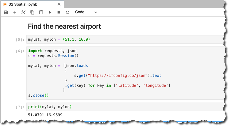
In your case, they should be different. And if you are on the VPN, then it might not even be your location at all. Adjust the location manually, if required ?
With these two variables
mylat and mylon properly set, we can now build a HANA DataFrame to query the nearest airport.dfh_nearport=(cchc
.table("PORTS")
.select("CODE", "DESC",
('New ST_Point("LON", "LAT").ST_SRID(4326)', "PORT_LOC"),
(
'New ST_POINT({lon}, {lat}).ST_SRID(4326).ST_Distance(New ST_Point("LON", "LAT").ST_SRID(4326))'
.format(lon=mylon, lat=mylat)
, "DIST_FROMME"
)
)
.sort("DIST_FROMME").
head(1)
)With this line of code we:
- select from the table
PORTStwo existing columnsCODE,DESCplus two calculated columns: PORT_LOCwith the spatial location of an airport- and the
DIST_FROMMEwith the distance in meters (that's the default unit of distance) from my location to an airport using the spatial reference IDSRID 4326. - Then we sort records by the distance column
- and select only one top record.
You can verify the generated
SELECT statement.dfh_nearport.select_statement
As we discussed already, the SQL in a HANA DataFrame is executed only when specific methods, like
collect() are called.dfp_nearport=dfh_nearport.collect()
dfp_nearport
So, the nearest airport is
WRO (as expected ?), located about 5.8 kilometers from me. But what is that array of bytes [1, 1, 0, 0, 0, 0, 0, 0, 192, 195, 226, 48, 64... as the location?Well, the spatial data is stored in a binary format. To be able to read it properly several methods in
hana_ml 2.6 have been extended with the geo_cols and srid optional properties, like sql().dfp_nearport=(cchc
.sql(
'''SELECT TOP 1
CODE, DESC,
New ST_Point(LON, LAT).ST_SRID(4326) as "PORT_LOC",
New ST_POINT(16.9599, 51.0791).ST_SRID(4326).ST_Distance(New ST_Point(LON, LAT).ST_SRID(4326)) as "DIST_FROMME"
FROM "PORTS"
ORDER BY "DIST_FROMME" ASC
'''.format(mylon, mylat),
geo_cols=["PORT_LOC"],
srid=4326
)
.collect())
display(dfp_nearport)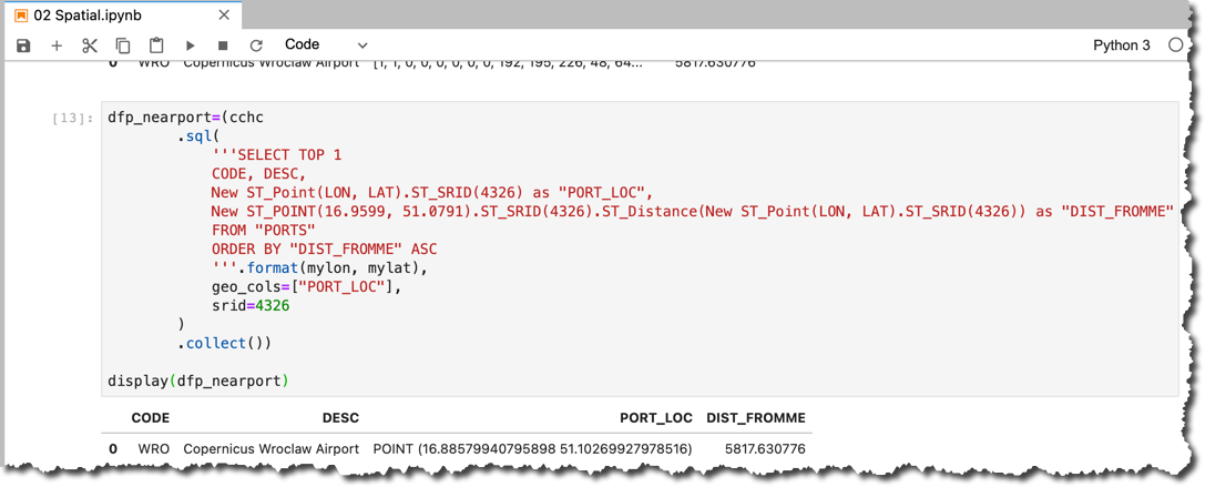
Now the airport's location is represented using the Well-Known Text (or WKT) value
POINT (16.88579940795898 51.10269927978516) that can be copied and pasted e.g. in http://geojson.io/ -> Meta -> Load WKT String to be displayed on the map.
"Isn't it possible to visualize spatial data now that we are using Python and Jupyter?" ask you. Absolutely! And we will get to that, but first, let us finish with the use of
geo_cols with HANA DataFrame.The next question would be what if you want to use HANA DataFrame methods to build the query, not embedded SQL, yet still, return the geospatial columns in the right format? This is where the trick, which I shared as a riddle in the first post, should help -- embedding dfh's
select_statement into SQL with geo_cols, like:dfp_nearport=(cchc
.sql(dfh_nearport.select_statement,
geo_cols={"PORT_LOC": 4326})
.collect()
)
display(dfp_nearport)
Last note here: check two different ways I used
geo_cols syntax. It can be:- either a dictionary combining a column name and SRID in one
geo_cols={"PORT_LOC": 4326}, - or -- convenient when you have multiple columns all with the same SRID -- a list of columns plus an SRID as two different parameters
geo_cols=["PORT_LOC"], srid=4326. In this example, it is a list of one element, but could be more.
Load input data with a geospatial column included
So far we had to calculate airport spatial points (locations) from
LAT and LON columns on the SAP HANA table PORT. It would be more convenient to create a column with this ST_GEOMETRY(4326) data type already at the data persistence.Let's do this now, but it means we need to repeat the step of reading and wrangling data from a CSV file using a Pandas dataframe
dfp_ports, the same as we did in 01 Dataframes.ipynb once again in the current Jupyter notebook.dfp_nodes=pd.read_csv('https://github.com/krlawrence/graph/raw/master/sample-data/air-routes-latest-nodes.csv')
dfp_ports=(
dfp_nodes[dfp_nodes['~label'].isin(['airport'])]
.drop(['~label','type:string','author:string','date:string'], axis=1)
.convert_dtypes()
)
dfp_ports.columns=(dfp_ports.columns
.str.replace('~','')
.str.replace(':.*','')
.str.upper()
)And once again we are creating (or rather re-creating SAP HANA table
PORTS thanks to force=True property) HANA DataFrame, indicating that a pair f columns LON and LAT are X and Y coordinates of a spatial point with Spatial Reference ID 4326.dfh_ports=dfh.create_dataframe_from_pandas(cchc,
dfp_ports, "PORTS",
geo_cols=[("LON", "LAT")],
srid=4326,
force=True
)This time a table in the database was created with the new
POINT_LON_LAT_GEO column, as seen by running a command:dfh_ports.columns
Now we can use this column to simplify the previous exploration of data, like finding the nearest airport!

Load spatial data from Esri shapefiles
Another great improvement in
hana_ml 2.6 is the ability to load Esri shapefiles, which is a very popular format to exchange geospatial data. I was very excited when saw this added functionality! I hope you are (or will be) too.We will use an old, but still very popular World Borders shapefile from the Thematic Mapping.
I am going to create a subfolder
Shapes and download the zipped file into that subfolder. This time I will do this right from my notebook's cell:!mkdir -p ./Shapes
!wget https://thematicmapping.org/downloads/TM_WORLD_BORDERS-0.3.zip -O ./Shapes/TM_WORLD_BORDERS-0.3.zip 
Let's use the new
create_dataframe_from_shapefile() method to persist the data in the SAP HANA table TM_WORLD_BORDERS. You can notice the use of geo_cols and srid here as well.dfh_countries = dfh.create_dataframe_from_shapefile(
connection_context=cchc,
shp_file='./Shapes/TM_WORLD_BORDERS-0.3.zip',
table_name="TM_WORLD_BORDERS",
geo_cols=["SHAPE"],
srid=4326
)and query the table to check your country, like
Poland in my case:dfh_countries.select("ISO2", "NAME", "SHAPE").filter("NAME='Poland'").collect()
As the last example let me show the HANA DataFrame's query joining two tables using the spatial predicate
ST_CoveredBy(). Please note the use of the alias() method to build the join of two HANA DataFrames dfh_ports and dfh_countries.How many airports are in Poland?
(

    dfh_ports.alias("P")

    .join

    (

        dfh_countries.filter("NAME='Poland'").alias("C"),

        condition='"P"."POINT_LON_LAT_GEO".ST_CoveredBy("C"."SHAPE")=1',

        select=["P.*"]

    )

).count()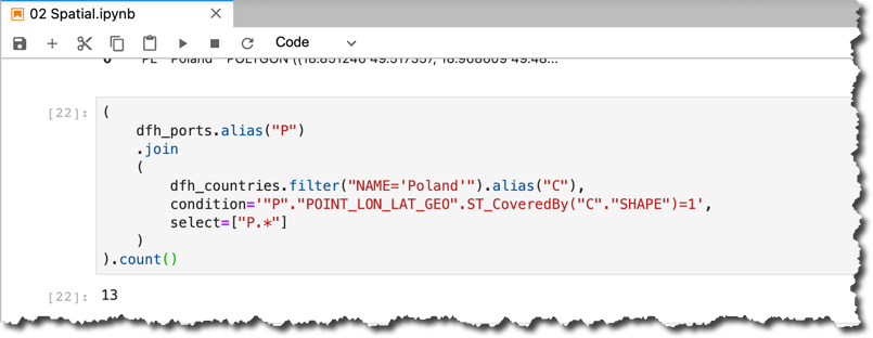
PS. And yes, I know there is a column
COUNTRY in the PORTS table, but I hope you get the point of this last overengineering effort ?You can find this notebook...
...in
hana-ml-samples repository: https://github.com/SAP-samples/hana-ml-samples/blob/main/Python-API/usecase-examples/multimodel-anal....A self-check riddle
Can you modify queries, using the distance unit other than the default meter? Two hints:
- Available units of measures are stored in SAP HANA in the table
"PUBLIC"."ST_UNITS_OF_MEASURE". - You can include the unit of measure as an optional parameter in the SAP HANA SQL method
ST_Distance().
As promised, we will focus on the visualization of the geospatial results in the next episode.
And stay healthy ❤️
-Vitaliy (aka @Sygyzmundovych)
PS. And if you read this on November 18th, then Happy GIS Day!
- SAP Managed Tags:
- SAP HANA Cloud,
- Python,
- SAP HANA,
- SAP HANA multi-model processing,
- SAP HANA Spatial,
- Big Data
Labels:
5 Comments
You must be a registered user to add a comment. If you've already registered, sign in. Otherwise, register and sign in.
Labels in this area
-
ABAP CDS Views - CDC (Change Data Capture)
2 -
AI
1 -
Analyze Workload Data
1 -
BTP
1 -
Business and IT Integration
2 -
Business application stu
1 -
Business Technology Platform
1 -
Business Trends
1,658 -
Business Trends
93 -
CAP
1 -
cf
1 -
Cloud Foundry
1 -
Confluent
1 -
Customer COE Basics and Fundamentals
1 -
Customer COE Latest and Greatest
3 -
Customer Data Browser app
1 -
Data Analysis Tool
1 -
data migration
1 -
data transfer
1 -
Datasphere
2 -
Event Information
1,400 -
Event Information
66 -
Expert
1 -
Expert Insights
177 -
Expert Insights
299 -
General
1 -
Google cloud
1 -
Google Next'24
1 -
Kafka
1 -
Life at SAP
780 -
Life at SAP
13 -
Migrate your Data App
1 -
MTA
1 -
Network Performance Analysis
1 -
NodeJS
1 -
PDF
1 -
POC
1 -
Product Updates
4,577 -
Product Updates
344 -
Replication Flow
1 -
RisewithSAP
1 -
SAP BTP
1 -
SAP BTP Cloud Foundry
1 -
SAP Cloud ALM
1 -
SAP Cloud Application Programming Model
1 -
SAP Datasphere
2 -
SAP S4HANA Cloud
1 -
SAP S4HANA Migration Cockpit
1 -
Technology Updates
6,873 -
Technology Updates
422 -
Workload Fluctuations
1
Related Content
- Multi-Model powering Intelligent Data Apps (2/3) in Technology Blogs by SAP
- AI-driven Public Urban Transport Optimization: implementation deep dive in Technology Blogs by SAP
- Develop a Machine Learning Application on SAP BTP - Data Science part in Technology Blogs by SAP
- Azure Machine Learning triggering calculations / ML in SAP Data Warehouse Cloud in Technology Blogs by SAP
- All you want to know on SAP HANA Cloud in Technology Blogs by SAP
Top kudoed authors
| User | Count |
|---|---|
| 40 | |
| 25 | |
| 17 | |
| 13 | |
| 7 | |
| 7 | |
| 7 | |
| 6 | |
| 6 | |
| 6 |