
- SAP Community
- Products and Technology
- Technology
- Technology Blogs by SAP
- Creating an SAC Geo Map from WebIDE (HDI) based Ca...
Technology Blogs by SAP
Learn how to extend and personalize SAP applications. Follow the SAP technology blog for insights into SAP BTP, ABAP, SAP Analytics Cloud, SAP HANA, and more.
Turn on suggestions
Auto-suggest helps you quickly narrow down your search results by suggesting possible matches as you type.
Showing results for
Product and Topic Expert
Options
- Subscribe to RSS Feed
- Mark as New
- Mark as Read
- Bookmark
- Subscribe
- Printer Friendly Page
- Report Inappropriate Content
07-21-2020
5:05 PM
In this blog post I will share how to create an SAP Analytics Cloud (SAC), Geo Map based on Calculation Views created within the WebIDE. These are Calc Views that reside within an HDI Container as Column Views.
For the official documentation please see the SAP Analytics Cloud Help
For the SAC Location Dimension to be identified, your calculation view needs the correct namespace. The namespace needs to be SAP_BOC_SPATIAL
There are two ways to different ways to achieve this.
Choose either the subfolder setting or the global setting.
1a. Specify the namespace at a specific sub-folder level
This can be done by creating a .hdinamespace file in a subfolder and that sub-folder will use that setting.
1b. Use the global project setting to append the hdinamespace setting as below
Warning, if you change an existing project using "ignore" then some re-work will be required.
With the Global namespace setting you the require a SAP_BOC_SPATIAL folder
SAP Analytics Cloud looks for location data inside the namspsace SAP_BOC_SPATIAL.
This should be created inside the WebIDE project src folder.
For SAC to visualise the location data, HANA must have the Spatial Reference 3857 available.
We can check this with the public synonym ST_SPATIAL_REFERENCE_SYSTEMS.
If you do NOT see the SRS_ID 3857 then you can execute the SQL below to add that
The location dataset must not contain duplicate values. To perform the correct join SAC requires a unique list of locations to ensure referential integrity of your model. This dataset will need latitude, longitude data and a field that joins to other Calc Views.
Here I have the table of UK Local Authorities, LAD2019_WKT, sorted on the field lad19cd, which I can see is unique.

We can now create a new dimensional Calculation View inside the SAP_BOC_SPATIAL folder. Notice how the Namespace field is populated with the required folder name.
The output column names need to be unique across the two calculation views that you are using with SAC. I therefore appended _geo to the end of the lad19cd and lad19nm.
Create Calculated Column of data type ST_POINT.
Using the fields "long" and "lat" we generate the ST_POINT column that SAP Analytics Cloud requires using the SRS 3857.
By specifying the "Key" column, SAC can identify which is the description field as it won't be the key.
We can Save and Build the Calculation View.
We can find our Calculation View as a Column View. Note how the name is prefixed with SAP_BOC_SPATIAL (the subfolder we created in step 2.)
We should data preview it to verify it works as expected. Note how the name is again prefixed with SAP_BOC_SPATIAL.
Open an existing SAC Model that will join to the fields exposed in the above model, in my case I can join on either lad19cd_geo or lad19nm_geo. Click the "Location Dimension" button.
We need to associate our Geo Dimensional Calc View with an existing calculation view.
The Location Identifier comes from an existing calculation view, this is the Attribute Column that joins to the Identifier for Mapping column coming from the step 5 "Geo Dimensional Calculation View". In my case Area_code joins to lad19cd_geo. This would be a 1:1 or many:1 with the many coming from the existing calculation view.
The final test is to create a Geo Map using this model to verify both the data and locations are displayed correctly on the map.
Spatial data has become more prevalent within the Enterprise, using SAP Analytics Cloud with HANA is a convenient way to visual this. From this blog post you can understand how SAP Business Application Studio or WebIDE based Calculation Views from HANA or HANA Cloud can be consumed live.
Pre-requisites
- HANA Cloud / HANA On-Prem with XSA
- Live Connection from SAC to HANA
- Dataset with Latitude and Longitude
- HDI Calculation Views (created via Business Application Studio or WebIDE)
Required Steps
- Create SAP_BOC_SPATIAL namespace
- Spatial Reference 3857
- Location Data
- Create Geo Dimensional Calculation View with ST_POINT
- Associate Calc Views in SAP Analytics Cloud Model
For the official documentation please see the SAP Analytics Cloud Help
1. Create SAP_BOC_SPATIAL namespace
For the SAC Location Dimension to be identified, your calculation view needs the correct namespace. The namespace needs to be SAP_BOC_SPATIAL
There are two ways to different ways to achieve this.
Choose either the subfolder setting or the global setting.
1a. Specify the namespace at a specific sub-folder level
This can be done by creating a .hdinamespace file in a subfolder and that sub-folder will use that setting.

Figure 1a: Subfolder Project Setting db/src/calc_views/Spatial
{

    "name": "SAP_BOC_SPATIAL",

    "subfolder": "ignore"

}
1b. Use the global project setting to append the hdinamespace setting as below

Figure 1b: Global Project Setting db/src/.hdinamespace
"subfolder": "append"Warning, if you change an existing project using "ignore" then some re-work will be required.
With the Global namespace setting you the require a SAP_BOC_SPATIAL folder
SAP Analytics Cloud looks for location data inside the namspsace SAP_BOC_SPATIAL.
This should be created inside the WebIDE project src folder.

Figure 2: SAP_BOC_SPATIAL folder
3. Spatial Reference 3857
For SAC to visualise the location data, HANA must have the Spatial Reference 3857 available.
We can check this with the public synonym ST_SPATIAL_REFERENCE_SYSTEMS.

Figure 3: ST_SPATIAL_REFERENCE_SYSTEMS - 3857
If you do NOT see the SRS_ID 3857 then you can execute the SQL below to add that
CREATE SPATIAL REFERENCE SYSTEM "WGS 84 / Pseudo-Mercator" IDENTIFIED BY 3857 TYPE PLANAR

SNAP TO GRID 1e-4

TOLERANCE 1e-4

COORDINATE X BETWEEN -20037508.3427892447 AND 20037508.3427892447 COORDINATE Y BETWEEN -19929191.7668547928 AND 19929191.766854766 ORGANIZATION "EPSG" IDENTIFIED BY 3857

LINEAR UNIT OF MEASURE "metre"

ANGULAR UNIT OF MEASURE NULL POLYGON FORMAT 'EvenOdd'

STORAGE FORMAT 'Internal'

DEFINITION 'PROJCS["Popular Visualisation CRS / Mercator",GEOGCS["Popular Visualisation CRS",DATUM["Popular_Visualisation_Datum",SPHEROID["Popular Visualisation Sphere",6378137,0,AUTHORITY["EPSG","7059"]],TOWGS84[0,0,0,0,0,0,0],AUTHORITY[ "EPSG","6055"]],PRIMEM["Greenwich",0,AUTHORITY["EPSG","8901"]],UNIT["degree", 0.01745329251994328,AUTHORITY["EPSG","9122"]],AUTHORITY["EPSG","4055"]],UNIT[ "metre",1,AUTHORITY["EPSG","9001"]],PROJECTION["Mercator_1SP"],PARAMETER["cen tral_meridian",0],PARAMETER["scale_factor",1],PARAMETER["false_easting",0],PA RAMETER["false_northing",0],AUTHORITY["EPSG","3785"],AXIS["X",EAST],AXIS["Y", NORTH]]'

TRANSFORM DEFINITION '+proj=merc +a=6378137 +b=6378137 +lat_ts=0.0 +lon_0=0.0 +x_0=0.0 +y_0=0 +k=1.0 +units=m +nadgrids=@null

+wktext +no_defs'
4. Location Data
The location dataset must not contain duplicate values. To perform the correct join SAC requires a unique list of locations to ensure referential integrity of your model. This dataset will need latitude, longitude data and a field that joins to other Calc Views.
Here I have the table of UK Local Authorities, LAD2019_WKT, sorted on the field lad19cd, which I can see is unique.
Figure 4: Location Dataset
5. Create Geo Dimensional Calculation View with ST_POINT
We can now create a new dimensional Calculation View inside the SAP_BOC_SPATIAL folder. Notice how the Namespace field is populated with the required folder name.

Figure 5: New Dimensional Calc View, notice the Namespace: SAP_BOC_SPATIAL
The output column names need to be unique across the two calculation views that you are using with SAC. I therefore appended _geo to the end of the lad19cd and lad19nm.

Figure 6: Location Dimensional Calculation View
Create Calculated Column of data type ST_POINT.
Using the fields "long" and "lat" we generate the ST_POINT column that SAP Analytics Cloud requires using the SRS 3857.
ST_Transform(ST_GeomFromText('POINT(' || "long" || ' ' || "lat" || ')', 4326),3857)
Figure 7: Calculated Column, LOCAL_AUTHORITY_GEO ST_POINT
By specifying the "Key" column, SAC can identify which is the description field as it won't be the key.

Figure 7.1: Specify the Key Field
We can Save and Build the Calculation View.

Figure 8: Build Calculation View
We can find our Calculation View as a Column View. Note how the name is prefixed with SAP_BOC_SPATIAL (the subfolder we created in step 2.)

Figure 9: Database Explorer Column View
We should data preview it to verify it works as expected. Note how the name is again prefixed with SAP_BOC_SPATIAL.

Figure 10: Data Preview of Local Authority Calc View
6. Associate Calc Views in SAP Analytics Cloud Model
Open an existing SAC Model that will join to the fields exposed in the above model, in my case I can join on either lad19cd_geo or lad19nm_geo. Click the "Location Dimension" button.

Figure 11: Open Existing SAC HANA Model
We need to associate our Geo Dimensional Calc View with an existing calculation view.
The Location Identifier comes from an existing calculation view, this is the Attribute Column that joins to the Identifier for Mapping column coming from the step 5 "Geo Dimensional Calculation View". In my case Area_code joins to lad19cd_geo. This would be a 1:1 or many:1 with the many coming from the existing calculation view.

Figure 12: Create Location Dimension
The final test is to create a Geo Map using this model to verify both the data and locations are displayed correctly on the map.
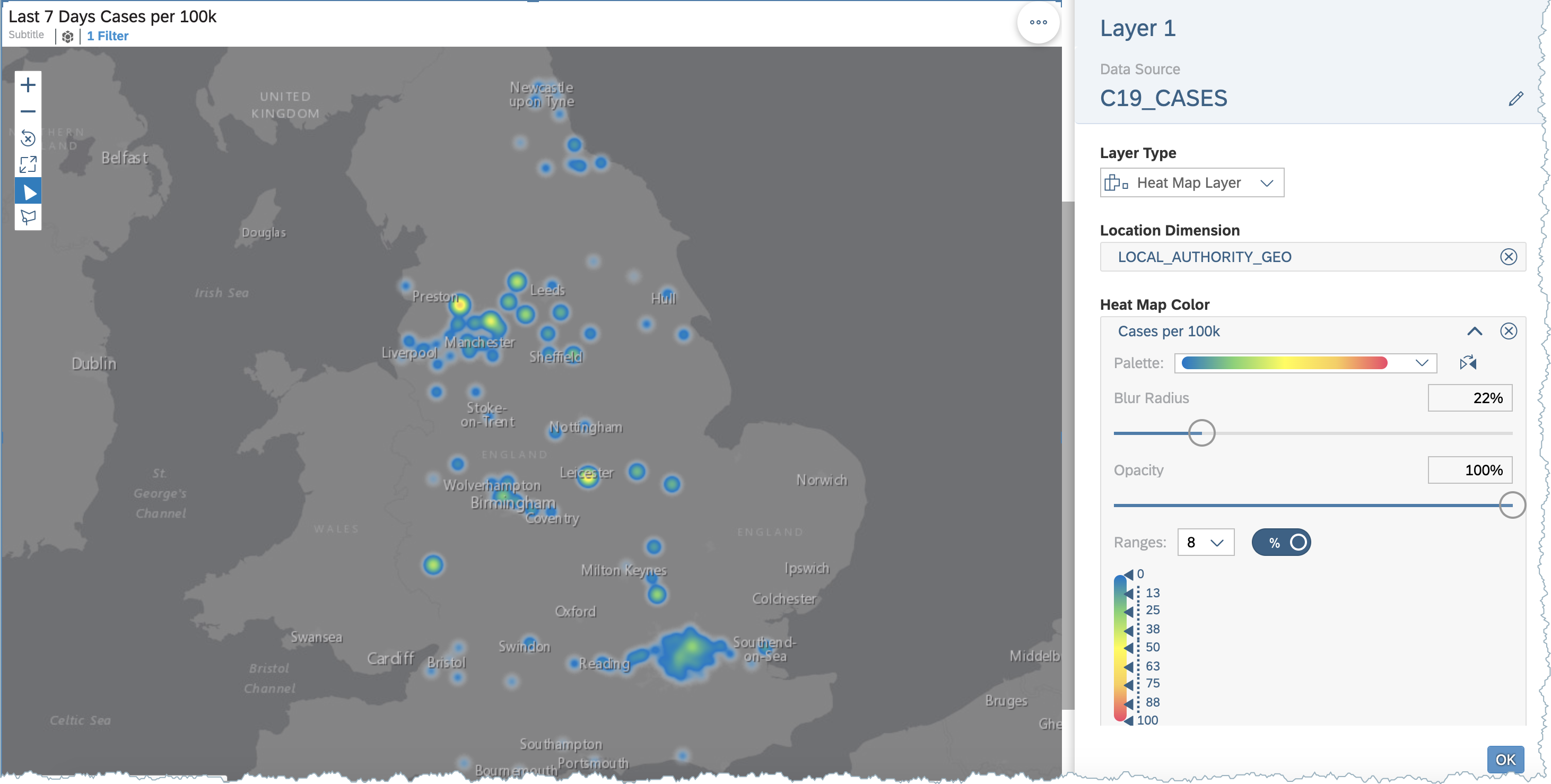
Figure 13: SAP Analytics Cloud Geo Map
Conclusion
Spatial data has become more prevalent within the Enterprise, using SAP Analytics Cloud with HANA is a convenient way to visual this. From this blog post you can understand how SAP Business Application Studio or WebIDE based Calculation Views from HANA or HANA Cloud can be consumed live.
- SAP Managed Tags:
- SAP Analytics Cloud,
- SAP HANA Cloud,
- SAP HANA,
- SAP HANA Spatial
Labels:
33 Comments
You must be a registered user to add a comment. If you've already registered, sign in. Otherwise, register and sign in.
Labels in this area
-
ABAP CDS Views - CDC (Change Data Capture)
2 -
AI
1 -
Analyze Workload Data
1 -
BTP
1 -
Business and IT Integration
2 -
Business application stu
1 -
Business Technology Platform
1 -
Business Trends
1,658 -
Business Trends
92 -
CAP
1 -
cf
1 -
Cloud Foundry
1 -
Confluent
1 -
Customer COE Basics and Fundamentals
1 -
Customer COE Latest and Greatest
3 -
Customer Data Browser app
1 -
Data Analysis Tool
1 -
data migration
1 -
data transfer
1 -
Datasphere
2 -
Event Information
1,400 -
Event Information
66 -
Expert
1 -
Expert Insights
177 -
Expert Insights
298 -
General
1 -
Google cloud
1 -
Google Next'24
1 -
Kafka
1 -
Life at SAP
780 -
Life at SAP
13 -
Migrate your Data App
1 -
MTA
1 -
Network Performance Analysis
1 -
NodeJS
1 -
PDF
1 -
POC
1 -
Product Updates
4,577 -
Product Updates
344 -
Replication Flow
1 -
RisewithSAP
1 -
SAP BTP
1 -
SAP BTP Cloud Foundry
1 -
SAP Cloud ALM
1 -
SAP Cloud Application Programming Model
1 -
SAP Datasphere
2 -
SAP S4HANA Cloud
1 -
SAP S4HANA Migration Cockpit
1 -
Technology Updates
6,873 -
Technology Updates
421 -
Workload Fluctuations
1
Related Content
- WebIDE: Extending Create Purchase Requisition New (F1643A) in Technology Q&A
- SAC - Add Row total to Dimension Subtotal? in Technology Q&A
- SAP Sustainability Footprint Management: Q1-24 Updates & Highlights in Technology Blogs by SAP
- Linear programming in ABAP. Simplex method. Find optimised BOM in Technology Blogs by Members
- Native HANA Information Views on Source system S4/HANA. in Technology Q&A
Top kudoed authors
| User | Count |
|---|---|
| 38 | |
| 25 | |
| 17 | |
| 13 | |
| 7 | |
| 7 | |
| 7 | |
| 7 | |
| 6 | |
| 6 |