
- SAP Community
- Products and Technology
- CRM and Customer Experience
- CRM and CX Blogs by Members
- SAP Forecasting with UDF (Unified Demand Forecast)
CRM and CX Blogs by Members
Find insights on SAP customer relationship management and customer experience products in blog posts from community members. Post your own perspective today!
Turn on suggestions
Auto-suggest helps you quickly narrow down your search results by suggesting possible matches as you type.
Showing results for
maciej_jarecki
Contributor
Options
- Subscribe to RSS Feed
- Mark as New
- Mark as Read
- Bookmark
- Subscribe
- Printer Friendly Page
- Report Inappropriate Content
07-13-2020
6:44 AM
Forecast for Retail industry
In SAP landscape there is a number of forecasting approaches. Starting with the simplest one which is executing forecast in S/4 based on consumption of goods and then taking them to Replenishment run. Next inbuild tool is to use multistep POS inbound replenishment process which is as well executed on S/4. The difference between two is that first one is based on consumption of goods IM which in Retail comes from GI of related to sales in stores transactions and the second one is based on POS recorded sales.
Beside inbuilt tools there is as well very often used forecasting external tool Forecast and Replenishment (F&R). The application is part of the SAP SCM solution and I assume it takes a lot of feature for calculation from SAP APO.
The last one tool fully dedicated to Retail industry is SAP Unified Demand Forecast (UDF). This application resides on SAP CAR and use very powerful Hana in-memory calculation and model of Bayesian regression. This forecasting tool is dedicated for Retail and fashion industry taking into account those industries specific aspects like prepack, sets articles, generic-variant relationship articles and dependencies between sites.
Step by step theory explanation
First of all please treat this article as an insight into the topic of forecasting with UDF as the scope of functionality and configuration can be a content for numbers of books.
Process of forecasting starts always with modelling that as a result creates a model of our data considering number of factors like seasons, trends, price impact etc. Modeling functionality tries to explain provided data to each DIF (demand influencing factor) and evaluate weight of it on the model.
Next step is to execute forecast. Forecasting use the results from modeling and given inputs such as planned promotions and prices. UDF can predict the effects of similar DIF occurrences in the future and derive from those the future demand.
Both activities can be executed in a number of variances from a product and location ranges point of view. Quite often we have new version of a product which doesn’t have yet sales history or new store opening with same situation. In this case either planning is done using data of reference product or both article hierarchies or stores dependencies are used.
- Aggregation: If your historical sales data at the product location level is sparse, demand influencing factors (DIFs) can be better detected at aggregate levels. In this case first run modeling on the aggregated data. Then results of aggregated modeling and forecasting increase baseline of and forecast at the product location level.
- Hierarchical priors: Configure the calculation of hierarchical priors to enhance the modeling of products for which little or no historical sales data or promotional data is available. With hierarchical priors, such products can “inherit” existing modeling results from suitable existing products along the hierarchies (product hierarchies, location hierarchies, relationships between generic products and their variants).
Due to the fact that forecasting is rather expert mode task which require high level of configuration and statistical knowledge not every change of any of parameters should be reflected in production outcome. In UDF we have an option to choose one of three modes when executing modeling of forecasting.
- Production mode: This is the default mode. You can schedule the run or execute it directly and the results are persisted in the database as new modeling or forecasting results.
- Diagnostic mode: This mode is for diagnostic evaluations and forecast analyses You specify a diagnostic ID for each diagnostic job that you want to run in situation when you want to adjust some parameters and test the flow and see results of potential changes in configuration. Example could be set decomposition of DIF in production environment and see the results.
- What-if forecast: You can trigger the run on demand. The results are provided to the consuming application as requested (for example, to SAP Promotion Management). What-if forecasts are frequently used during planning because they allow you to gauge the impact of a particular course of action that may or may not be executed in the future (such as a planned offer).
Source of data - UDF supports various time series sources (such as point-of-sale data, consumption data, or sales orders). The most commonly used in POS data which can be as well enhance with Sales orders data coming from other sales channels (like e-commerce). Data can have granularity of day or week and it’s always recommended to provide last two years of historical data than system can distinguish seasons, trends etc.
As a summary for forecasting with UDF following activates need to be executed:
- Run initial modeling – optional
- Run Hierarchical priors modeling - optional
- Run hierarchy or product/location modeling -mandatory
- Run forecasting for product/location or hierarchy assignment - mandatory
Simple scenario configuration – technicalities
As a simple scenario I would like to check which models are available as standard in UDF plus with diagnostic mode see the influence of changing some standard parameters.
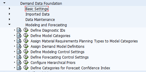
All configuration is done in CAR under node SPRO -> SAP CAR -> Demand Data Foundation -> Modeling and Forecasting.
The fist step is to create Diagnostic ID that will be used for testing of modeling and forecasting parameters adjustments.

When Diagnostic ID has been defined the next step is to configure which source of data is used in our model and which model it self will be used.

- Time series in my case (and most of them I assume) is data coming from POS system.
- Aggregation profile in my case is not used but as described before it can help to group articles for more accurate results like T-Shirt is sold in different colors and sizes and modeling on aggregated level will give for sure more precious figures.
- Model Category is used only if you want to make extra split of modeling per MRP type.
- Model definition is the most important parameter that describes which model definition is used and how decomposition to particular system or customer DIFs are taken into account to calculate model values. There is much more to configure under each model definition then only System or Customer DIFs.
In standard following three type are delivered CPG, RTL, RTLSDP.

After selecting model definition there is an option to set parameters that will for example influence system calculation or will help to investigate results of modeling
Number of parameters in both modeling and forecasting areas in quite significant and some of them require deep statistical knowledge. Following example of ones that I setup in my scenario.
Modeling:
- MOD_COV_REDUCED – ‘ ‘ depends how covariance matrix is generate. Empty value is a default one and means full.
- MOD_OUTPUT_COV – ‘X’ required for FCI calculation or hierarchical priors
- MOD_DAYS_IN_PERIOD – number of days of sales history that are taken into account for calculation of model data.
- MOD_OOSD_MIN_LEN – minimum number of days without any sales so the system can treat it as out of stock situation.
- MOD_OUTPUT_DECOMP – ‘X’ allows decomposition of each DIF influence on the model. Results are stored in table /DMF/UMD_TSD.
- MOD_OUTPUT_TS – ‘X’ Controls the calculation and output of model fit and traceability information in the /DMF/UMD_TS table.
- MOD_TD_ERROR_VARIANCE – ‘X’ Controls the calculation and output of time-dependent error variances for modeling. A separate error variance is calculated for each demand influencing factor.
Forecasting:
- FC_HZN_DUR_DAYS - Number of days to forecast
- FC_OUTPUT_DECOMP - Enable the demand decomposition if you wish to output forecasted unit per demand influencing factor (DIF). Results are stored in /DMF/UFC_TSD table.
- FC_OUTPUT_FCI - Controls the calculation of the forecast confidence index (FCI).
- FC_OUTPUT_TRACE - Controls the output of additional trace information like product prices, product listings which are stored in /DMF/UFC_TRC table.
- FC_TD_ERROR_VARIANCE – ‘X’ Controls the calculation and output of time-dependent error variances for forecasting. A separate error variance is calculated for each demand influencing factor.
When modeling and forecasting parameters have been set and assigned to option diagnostic id which is a link to Model definition used. Model definition contains a list of DIF that are used to calculate component of final values of model and follow up forecast.

Each DIF assigned to model has parameters that describes if used in a model (DIF Mode) and how they are grouped (DUS Mapping). Additionally DIF has default parameters used in Model and Forecast calculation.

Beside presented only basic properties of DIF and it usage in model and forecast calculation number of configurable settings that can influence calculation is for example weight of each weekday or how before or after holiday time period influence calculation results.
Result
Below are presented results of modeling run with three different standard models on the same data probe (two years of historical sales).
CPG – SAP Retail Weekly Demand Model Definition for Yearly Seasonality with ACV Active

Calculated value for 13/02 is 5.065 PC
RTL - SAP Retail Demand Model Definition for Yearly Seasonality

Calculated value for 13/02 is 4.935 PC
RTLSDP - SAP Retail Demand Model Definition for Short Seasonal Patterns

Calculated value for 13/02 is 5.688 PC
Results of modeling and forecasting are store respectively in table /DMF/UMD_TS and /DMF/UFC_TS where value of FCI parameter (for forecast) and MOD VAL (for modeling) are stored. First one describes how amount and quality of the statistical input data based on which the forecast was generated and the second one measure calculated model fit to the input data.
If decomposition has been activated result of each DIF calculation is stored in /DMF/UMD_TSD table. For RTL model (middle screen) model value is 4.935 PC and has been calculated based on values of DIF:
- SYS:CAL:TRND = - 5,28373 (DUS Mapping – BASE)
- SYS:CAL:WK:DAY = - 0,10121 (DUS Mapping – BASE)
- SYS:CAL:YR:HRM = - 14,96814 (DUS Mapping – SEASON)
- SYS:INT = 26,90757 (DUS Mapping – BASE)
- SYS:PRC = - 1,61955 (DUS Mapping – PRICE)
Based on each calculated DIF and it assignment to group BASE is 21,523 PC (blue on the model) SEASON – 14,968 PC ( orange on the model) and PRICE -1,62 PC (Dark blue on the model)
Customer DIF
The best way to compare result of modeling and forecasting is to set forecasting start day in the not faraway past where enough historical data is available and compare obtained results with real data. If planner has observed that model is not full describing data that is option to incorporate own DIF. Custom DIF is either Boolean or metric. First type can have two value, true or false. Second one can have values according to DIF definition.
Own DIF definition is created with new entry to /DMF/V_DIF where beside the type as well validity level is assigned. The next step is to add DIF to the model definition by editing cluster /DMF/VC_MOD_DEF. Import of data for Custom DIF can be done function module /DMF/MDIF_USER_DIF_INBOUND and then processing of staging table.

Hope this article gives a bit of light on UDF topic.
- SAP Managed Tags:
- SAP Customer Activity Repository,
- SAP Forecasting and Replenishment
12 Comments
You must be a registered user to add a comment. If you've already registered, sign in. Otherwise, register and sign in.
Labels in this area
-
ABAP
1 -
API Rules
1 -
c4c
1 -
CAP development
1 -
clean-core
1 -
CRM
1 -
Custom Key Metrics
1 -
Customer Data
1 -
Determination
1 -
Determinations
1 -
Introduction
1 -
KYMA
1 -
Kyma Functions
1 -
open SAP
1 -
RAP development
1 -
Sales and Service Cloud Version 2
1 -
Sales Cloud
1 -
Sales Cloud v2
1 -
SAP
1 -
SAP Community
1 -
SAP CPQ
1 -
SAP CRM Web UI
1 -
SAP Customer Data Cloud
1 -
SAP Customer Experience
1 -
SAP CX
1 -
SAP CX extensions
1 -
SAP Integration Suite
1 -
SAP Sales Cloud v2
1 -
SAP Service Cloud v2
1 -
SAP Service Cloud Version 2
1 -
Service and Social ticket configuration
1 -
Service Cloud v2
1 -
side-by-side extensions
1 -
Ticket configuration in SAP C4C
1 -
Validation
1 -
Validations
1
Related Content
- Maximize Results and Drive Sustainability in Fashion Retail with SAP and GK AIR Dynamic Pricing in CRM and CX Questions
- Get Started with Embedded SAP Analytics Cloud in SAP Sales & Service Cloud (C4C) in CRM and CX Blogs by SAP
- Navigating the Modern Sales Landscape: The AI Advantage, SAP Sales Cloud Intelligent Sales Add-on in CRM and CX Blogs by SAP
- Unleashing Customer Insights: SAP CDP for Retail in CRM and CX Blogs by SAP
- Aggregated Forecast in combination with user DIF; CAR-System in CRM and CX Questions
Top kudoed authors
| User | Count |
|---|---|
| 1 | |
| 1 | |
| 1 | |
| 1 | |
| 1 |