
- SAP Community
- Products and Technology
- Technology
- Technology Blogs by SAP
- Fuzzy Matching Reimagined with Data Science - Part...
Technology Blogs by SAP
Learn how to extend and personalize SAP applications. Follow the SAP technology blog for insights into SAP BTP, ABAP, SAP Analytics Cloud, SAP HANA, and more.
Turn on suggestions
Auto-suggest helps you quickly narrow down your search results by suggesting possible matches as you type.
Showing results for
former_member65
Explorer
Options
- Subscribe to RSS Feed
- Mark as New
- Mark as Read
- Bookmark
- Subscribe
- Printer Friendly Page
- Report Inappropriate Content
07-01-2020
3:42 PM
Ever looked for matches that were less than 100% perfect? Key based matches not working for you? Until a few years ago, fuzzy matching was the only answer we had. Today, data science algorithms are breaching the boundaries of the “possible”. Find out how we used algorithms typically applied to document similarity to solve the traditional fuzzy matching problem using SAP Data Intelligence & SAP Analytics Cloud.
Recently we were approached by a municipality in India for an easy way to match profiles across official covid-19 case lists. The govt officers were eyeballing the data and manually finding records of individuals that overlapped between the positive case lists and the quarantine / de-quarantine lists. This was of course time consuming and a typical clarion call for automation. The traditional approach for this is a process called fuzzy matching, which would involve matching the profiles on the basis of Name, Gender, Age and Address much like a join, but where the constraints are relaxed to have a match that is less than 100% pure. It’s similarity to a join, in the context of a string based comparison, implies processing time will expand exponentially with the size of the database.
Until some years ago, this would have been the unavoidable drudgery that we would have to plough on through. But not anymore. The idea of TF-IDF (term frequency, inverse document frequency) stems from the need to highlight how important a word is to a document in a collection or a corpus. For ex. In documents to do with wild life conservation, you can expect a set of keywords to occur more often than say in documents to do with supply chain. But in large documents the frequency of occurrence can simply be due to its size. So we find a way to control for document size, and define TD-IDF as the number of times a word appears in a document, offset by number of documents in the corpus that contain the word. This is a technique typically applied in searches for document similarity in its general form. We can easily extend it to user profiles, especially in the case of names and addresses.
We were handed 3 csv files containing records of covid-19 positive, quarantined and de-quarantined cases respectively. There were certain columns which were present in all 3 csv files but due to the manual nature of data collection they were mostly in different formats. Had data been collected by a single vendor in the same format, the job of collating all this data from these sources would have been a simple join on the common columns. Since real world scenarios are far from ideal, we need to jump through hoops to get the files ready before modelling.
Step 01: Data Pre-processing
Clean and homogenize data, so the disparate files can blend seamlessly.
- Convert all fields to upper case
- Delete the empty columns and clear the rows with null values in more than 8 columns.

- Homogenize frequently occurring keywords (chd to Chandigarh, Blk to Block, Hs to House, etc.)
- Impute missing values
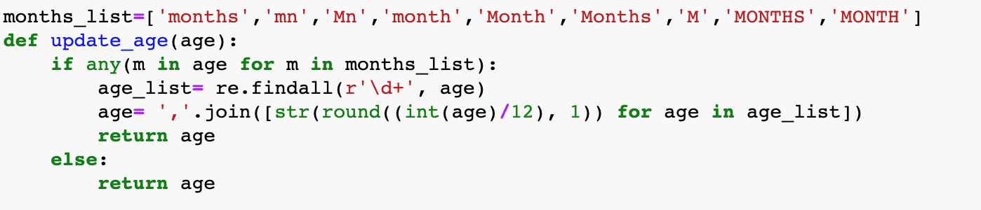
- Clean data type inconsistencies (in dates, age, etc.)
- If Sector number is missing in the address field, add it in from the Sector column.

- Remove or replace special characters, as required. The ‘&’ symbol is replaced by ‘and’ and consecutive spaces are replaced with a single space. This string is then used to create n-grams of length 3.

- These n-grams cannot be directly used in models. Hence, we convert these strings into a matrix of tf-idf values. Although this is generally used on words, we can use this on n-grams as well.

- Apart from this, we extracted all unique sector records and geocoded them to retrieve the latitude and longitude values which we used later to show the sector wise aggregated numbers on the SAP Analytics Cloud Dashboard.
Step 02: Build Models
Cosine Similarity
Cosine similarity is a very popular technique used to find similarity between two vectors. In the current scenario, we find the similarity between two string vectors. The function used to calculate cosine similarity is shown below.

Nearest Neighbor
In this approach, we compare a record from one set with all the records in the other set and obtain a similarity score. The function below takes tf-idf matrix that was created earlier as input.

Step 03: Post Processing
- Both these models are applied separately for name and address. We filter in records that have a similarity score above a defined threshold value, rejecting low similarity matches. In our case, we have used a threshold value of 0.55.
- We then do an inner join on the results to just retrieve cases for which name and address matches point to the same records. We also store the outer join results on top of the inner join results to ensure that we are able to cover cases where just one of the two columns match. These results will then be shown to the data steward for review.
- Apart from the original columns, two additional columns are inserted into the final csv that is generated. One column denotes the method used to calculate the similarity score and the second column defines if review is needed or not. Review needed flag is set when both the algorithms return different matches and if the similarity scores of either of them are not very satisfactory.
- We create a file called Bridge that contains the complete source records, source ID, similarity score & match ID. This will be reviewed by a steward to determine if the matched groups are acceptable or not. We also create a file called Master which contains the best profile or golden record from all members within each matched group.
In this blog, we have shown a step by step approach on how we cleaned the data, built models using it and how we later aggregated the results from the models so that it can then be presented to the stakeholders. In Part 2 of this blog post, we describe how these models were scheduled and deployed in SAP Data Intelligence.
- SAP Managed Tags:
- Machine Learning,
- SAP Analytics Cloud,
- SAP Data Intelligence
Labels:
You must be a registered user to add a comment. If you've already registered, sign in. Otherwise, register and sign in.
Labels in this area
-
ABAP CDS Views - CDC (Change Data Capture)
2 -
AI
1 -
Analyze Workload Data
1 -
BTP
1 -
Business and IT Integration
2 -
Business application stu
1 -
Business Technology Platform
1 -
Business Trends
1,661 -
Business Trends
86 -
CAP
1 -
cf
1 -
Cloud Foundry
1 -
Confluent
1 -
Customer COE Basics and Fundamentals
1 -
Customer COE Latest and Greatest
3 -
Customer Data Browser app
1 -
Data Analysis Tool
1 -
data migration
1 -
data transfer
1 -
Datasphere
2 -
Event Information
1,400 -
Event Information
64 -
Expert
1 -
Expert Insights
178 -
Expert Insights
270 -
General
1 -
Google cloud
1 -
Google Next'24
1 -
Kafka
1 -
Life at SAP
784 -
Life at SAP
11 -
Migrate your Data App
1 -
MTA
1 -
Network Performance Analysis
1 -
NodeJS
1 -
PDF
1 -
POC
1 -
Product Updates
4,578 -
Product Updates
323 -
Replication Flow
1 -
RisewithSAP
1 -
SAP BTP
1 -
SAP BTP Cloud Foundry
1 -
SAP Cloud ALM
1 -
SAP Cloud Application Programming Model
1 -
SAP Datasphere
2 -
SAP S4HANA Cloud
1 -
SAP S4HANA Migration Cockpit
1 -
Technology Updates
6,886 -
Technology Updates
395 -
Workload Fluctuations
1
Related Content
- SAP Datasphere in Simple terminology, its Strategy and Benefits. in Technology Blogs by Members
- Leveraging Artificial Intelligence in Finance, Supply Chain, and ERP: An In-Depth Guide in Technology Blogs by SAP
- SAUG Conference Brisbane 2023 in Technology Blogs by Members
- The 49ers Turn to Real-time Data to Deliver Superior Home Game Experiences for 70k+ Fans in Technology Blogs by SAP
- Expert Guided Implementation – The Security Optimization Service EGI: Simple and Powerful in Technology Blogs by SAP
Top kudoed authors
| User | Count |
|---|---|
| 11 | |
| 10 | |
| 10 | |
| 9 | |
| 8 | |
| 7 | |
| 7 | |
| 7 | |
| 7 | |
| 6 |