
- SAP Community
- Products and Technology
- Enterprise Resource Planning
- ERP Blogs by Members
- SAP S/4HANA DDMRP – Buffer Profiles, Product and L...
Enterprise Resource Planning Blogs by Members
Gain new perspectives and knowledge about enterprise resource planning in blog posts from community members. Share your own comments and ERP insights today!
Turn on suggestions
Auto-suggest helps you quickly narrow down your search results by suggesting possible matches as you type.
Showing results for
hrishi_pendse
Explorer
Options
- Subscribe to RSS Feed
- Mark as New
- Mark as Read
- Bookmark
- Subscribe
- Printer Friendly Page
- Report Inappropriate Content
06-29-2020
12:10 PM
In this blog, I have tried to throw some light on Buffer profiles in DDMRP and how to use Product and Lead time Classification tools fine tune the key parameters from buffer profile, with SAP S/4HANA 1809 on-premise version.
Sources:
Buffer Profiles
In DDMRP, Buffer Profiles play a very important role in determining the level of Buffer Inventory that you need to maintain for materials. As a part of configuration, you need to maintain some key parameters for Buffer profiles, which will control the Buffer Inventory.
Here, you need to maintain the variability factor and lead time factor, which will be used to calculate Buffer Levels for materials. For Variability and Lead time factors respectively, SAP has given values initially for Buy, Make and Transfer as:
Low / Short = 0.3
Medium = 0.5 and
Hing / Long = 0.8
Apart from those, you can define your own values. Based on the results from your Product and Lead time Classifications (which are explained below), you can define your own values for these parameters, that are suitable for your organization.
Variability factor and Lead time factor are basically the multipliers that are used in the buffer calculation from the “Red” zone (explained below).
You would be defining the buffer profile based on 3 procurement types – Buy, Make and Transfer. Based on that, you can differentiate, what values you need to define for 'Variability factor' and 'Lead time factor'. They will decide the “Buffer levels” that you are supposed to maintain.
Buffer Sizing and Buffer Zones –
To calculate the buffer quantity for DDMRP relevant materials, system performs quantity calculations split into three different zones, layer top to bottom in order –
Anything above Green Zone is a Blue Zone (Quantity from blue zone is not calculated and considered as excess).
Buffer zones are dynamic in nature and system follows certain logic and uses formulas to determine the quantity of stock that each zone should contain, for a particular material. The sum of these three zones form the maximum level of Buffer Inventory.
Those quantities are typically calculated using “Average Daily Usage” based on the goods issues that is done for a material on day-to-day basis, Variability factor and Lead Time factor.
What is the basis of selecting the variability and lead time factor values? – If your lead time and variability are high, then you will need to keep more inventory in Red Zone and so, you can maintain high value for both variability and lead time factors. If your variability is low, then you can maintain low values for them.
For example, based on Average Daily Usage for a material and Decoupled lead time, system has calculated Red Zone as 200 and lead time factor that you have maintained is 0.3 – as the material has low lead time (decoupled lead time).
The definition of “low” is based on the lead time values that you get for different materials in your “maintain material classification” – so, let’s say – 3 days of delivery time may be low for your company, 4-10 days is medium and 11 days or above is high lead time. So, let’s say, for low, med and high, you have defined 0.3, 0.5 and 0.8 respectively as lead time factors for them.
So, system will calculate the “Red Base” = Yellow zone x Lead time factor → 200 x 0.3 = 60 as your Red Base.
These key parameters (Lead time and Variability factor), you may not get right at first time. You need perform several iterations before you get desired values based on your testing and experience from your organization. That is why DDMRP takes take time to reach certain maturity level, as all these parameters may need some fine tuning over period of time.
You will be getting the “Variability Indicator” and “Lead time Indicator” values from your classification of the data (classification tool). The classification tool will help you to define the variability and lead time indicator values as X – Low, Y – Medium, Z – High and E – Short, F – Medium, G – Long respectively.
So, with the combination of variability and lead time indicators and factors, system will decide the buffer levels.
Buffer Calculations
Source for the Formulas used below is: https://help.sap.com/viewer/e93a1ed5d8d9422faa3acd132b27e7ba/1709%20000/en-US
Note: Figure was created, referring to SAP documentation from – https://help.sap.com/viewer/e93a1ed5d8d9422faa3acd132b27e7ba/1709%20000/en-US
& the book – Demand Driven Material Requirements Planning (DDMRP) V2; by Carol Ptak, Chad Smith
Firstly, the system calculates Yellow Zone as:
Yellow Zone = Average Daily Usage x Decoupled Lead Time
The Top of Yellow Zone is nothing but your Reorder Point.
Then, using Yellow zone value, system determines the Red Base part as,
Red Base = Yellow Zone x Lead Time Factor
Next comes the Red Safety zone, which is calculated using Red Base as –
Red Safety = Red Base x Variability Factor
“Red Buffer Levels” are like the “Safety Stock”; and those will be defined by the variability factor and lead time factor.
Finally, system arrives to Green Zone Calculations as –
Green Zone = Maximum of [(Yellow Zone x Lead Time Factor) OR (Minimum Order Quantity) OR (Average Daily Usage x Order Cycle)]
Schedule Product Classification (DD)
This is the first App that you need to use when you start using DDMRP.
Product Classification is a tool that helps you to classify your materials based on certain conditions and then select which products are relevant for DDMRP. Although, this tool helps you to identify such materials, you can also use own experience from your organization to decide to choose materials for DDMRP, depending their behavior in the supply chain.
Here, you need to set up a job for this classification and along with other inputs, you should mention the number of days in the past, to tell the system, how long in the past, the system should consider historic data for product classification.
Source: SAP S/4HANA 1809 on premise version.
Next, you need to maintain the Threshold for values for ABC classification. In this, you typically maintain the classification for materials based on the percentage usage value and keep fine-tuning them over a period of time until you get desired results. For the number of days in the past that you have maintained, system will identify the goods issue amount (value) and then sort the materials in descending order and then categorize.
For example, let’s say, you have maintained A = 30%, B = 30% and C = 40%
and you have below materials with good issue values (in currency unit) –
Material M = 3000, Material N = 1500, Material O = 1400, Material P = 600, Material Q = 200
Material R = 1200, Material S = 1100, Material T = 100, and so on, with total of 15000 EUR value goods. So, based on the classification percentage, system will categorize the materials under A, B and C.
You have maintained A = 30%, B = 30% and C = 40%
Here, 30% of 15000 is 4500 EUR, which is forms your top range products – Material M and N – categorized under “A”, next 30% under B which are – material O, P R and S under and the rest of them under C.
Note that, instead of the product cost, system considers the total valued good issue for a particular material. That is, if two products – one with a high price and other with very low – have same value of goods issue, then system treats them equally. If the low-price material has higher good issue value than, the high-price material, then low price material may fall under category A and the one with high price, in category B or even C).
Then, you will be defining Thresholds for BOM Usage under PQR classification. In this, you will maintain high, medium and low values for material’s usage in BOM’s. For instance, if a particular material is used in 5 different BOM’s, then maybe it can be categorized under P (High usage), materials used in 3 BOMS are classified as Q (Medium usage) and anything < 3 is R (Low usage). This type of classification totally depends on what type of BOM structure you have in your organization. If the structure is huge, then maybe 50 can be High and 20 can be low for your organization.
Another important key parameter for classification is Threshold for Variability XYZ classification.
The variability for material is measured here based on the actual consumption of material based on actual demand. On a particular date, system takes into consideration the sum of Sales order quantity that is due, overdue and accepted order spikes to calculate actual demand.
Considering the time dependent actual demand, the material consumption may fluctuate between high to low consumption values.
Based on this fluctuation, you decide the variability for a material. Materials with higher variability will cause more issues in supply chain – either high inventories or stock-outs. Those materials should be monitored closely.
This variability is managed here with coefficient of variation. In S/4HANA DDMRP, it is typically calculated over the time interval that you have selected. For a material, system calculates Standard Deviation and Mean Deviation and then coefficient of variation for actual demand is derived as Standard Deviation / Mean Deviation.
So here, for example, you can set the thresholds as 0.1 as X (Low), 0.2 as Y (Medium) and anything > 0.2 as Z (High). Based on the thresholds that you set, system calculates the 'Variability' and classifies materials with High, Medium and Low Variability Factor.
You should consider the collective effect of ABC – PQR – XYZ classification to identify which materials you need to consider for DDMRP and monitor them closely. That means, material with combination of A-P-X is a critical material compared to C-P-Z combination of the above classification.
Note:Values used in above cases are not realistic and used for understanding the concept.
Lead Time Classification
Here also, system will consider the number of days in the past that you have mentioned.
In Lead time Classification App, you maintain the Threshold Values for Lead time in number of days for Make, Buy and Transfer.
Here, you have to maintain values for parameters – E (Short), F (Medium) and G (Long) in number of days. Based on the experience from your organization you need to identify what is short, medium and long lead time for materials. These parameters are not fixed and will vary from business to business and the nature of the business will have an impact on them.
You can see the results from your Product and Lead time classification in Mass Maintenance of Products (DD) App.
It will show you the classifications of products based on the threshold parameters for good issue values, variability coefficient, BOM usage and decoupled lead time as discussed above. You can use available filters on them to get a clear picture on critical materials.
Based the Variability (XYZ) and Lead time (EFG) classifications results, you may need to fine tune the values for Variability Factor and Lead time factor that you have maintained in your Buffer Profile configuration (Table: PPH_BF_PRFLDET_V), until DDMRP reaches certain maturity level to give desired results.
Along with Buffer Profile configuration, there is another import factor that we need to consider is – the qualified order spikes or the spiked in demand. The purpose to consider them is to protect your buffer inventory from irregularities in future consumption which was not taken into account, considering the current Lead time and Variability factors as seen above. However, I will cover this topic in an upcoming blog.
So, to conclude – I have tried to shed some light on - the Buffer Profiles configuration in SAP S/4HANA DDMRP, the concept behind Buffer Zones and how Buffer Profiles work in tandem with Product and Lead time classification tools.
Thanks for reading! Appreciate your feedback and comments.
Sources:
- https://help.sap.com/viewer/e93a1ed5d8d9422faa3acd132b27e7ba/1709%20000/en-US
- Demand Driven Material Requirements Planning (DDMRP) V2; by Carol Ptak(Author), Chad Smith
- https://www.demanddriveninstitute.com/
Buffer Profiles
In DDMRP, Buffer Profiles play a very important role in determining the level of Buffer Inventory that you need to maintain for materials. As a part of configuration, you need to maintain some key parameters for Buffer profiles, which will control the Buffer Inventory.

Figure 1: Maintain Buffer Profiles – Transaction SM30 - Table: PPH_BF_PRFLDET_V
Source: SAP S/4HANA 1809 on premise version
Here, you need to maintain the variability factor and lead time factor, which will be used to calculate Buffer Levels for materials. For Variability and Lead time factors respectively, SAP has given values initially for Buy, Make and Transfer as:
Low / Short = 0.3
Medium = 0.5 and
Hing / Long = 0.8
Apart from those, you can define your own values. Based on the results from your Product and Lead time Classifications (which are explained below), you can define your own values for these parameters, that are suitable for your organization.
Variability factor and Lead time factor are basically the multipliers that are used in the buffer calculation from the “Red” zone (explained below).
You would be defining the buffer profile based on 3 procurement types – Buy, Make and Transfer. Based on that, you can differentiate, what values you need to define for 'Variability factor' and 'Lead time factor'. They will decide the “Buffer levels” that you are supposed to maintain.
Buffer Sizing and Buffer Zones –
To calculate the buffer quantity for DDMRP relevant materials, system performs quantity calculations split into three different zones, layer top to bottom in order –
- Green Zone (Maximum Stock Level)
- Yellow Zone (Reorder Point Level)
- Red Zone, which is further divided in –
- Red Safety (Safety Stock)
- Red Base (Minimum Safety Stock)
Anything above Green Zone is a Blue Zone (Quantity from blue zone is not calculated and considered as excess).
Buffer zones are dynamic in nature and system follows certain logic and uses formulas to determine the quantity of stock that each zone should contain, for a particular material. The sum of these three zones form the maximum level of Buffer Inventory.
Those quantities are typically calculated using “Average Daily Usage” based on the goods issues that is done for a material on day-to-day basis, Variability factor and Lead Time factor.
What is the basis of selecting the variability and lead time factor values? – If your lead time and variability are high, then you will need to keep more inventory in Red Zone and so, you can maintain high value for both variability and lead time factors. If your variability is low, then you can maintain low values for them.
For example, based on Average Daily Usage for a material and Decoupled lead time, system has calculated Red Zone as 200 and lead time factor that you have maintained is 0.3 – as the material has low lead time (decoupled lead time).
The definition of “low” is based on the lead time values that you get for different materials in your “maintain material classification” – so, let’s say – 3 days of delivery time may be low for your company, 4-10 days is medium and 11 days or above is high lead time. So, let’s say, for low, med and high, you have defined 0.3, 0.5 and 0.8 respectively as lead time factors for them.
So, system will calculate the “Red Base” = Yellow zone x Lead time factor → 200 x 0.3 = 60 as your Red Base.
These key parameters (Lead time and Variability factor), you may not get right at first time. You need perform several iterations before you get desired values based on your testing and experience from your organization. That is why DDMRP takes take time to reach certain maturity level, as all these parameters may need some fine tuning over period of time.
You will be getting the “Variability Indicator” and “Lead time Indicator” values from your classification of the data (classification tool). The classification tool will help you to define the variability and lead time indicator values as X – Low, Y – Medium, Z – High and E – Short, F – Medium, G – Long respectively.
So, with the combination of variability and lead time indicators and factors, system will decide the buffer levels.
Buffer Calculations
Source for the Formulas used below is: https://help.sap.com/viewer/e93a1ed5d8d9422faa3acd132b27e7ba/1709%20000/en-US

Figure 2: Buffer Zones
Note: Figure was created, referring to SAP documentation from – https://help.sap.com/viewer/e93a1ed5d8d9422faa3acd132b27e7ba/1709%20000/en-US
& the book – Demand Driven Material Requirements Planning (DDMRP) V2; by Carol Ptak, Chad Smith
Firstly, the system calculates Yellow Zone as:
Yellow Zone = Average Daily Usage x Decoupled Lead Time
The Top of Yellow Zone is nothing but your Reorder Point.
Then, using Yellow zone value, system determines the Red Base part as,
Red Base = Yellow Zone x Lead Time Factor
Next comes the Red Safety zone, which is calculated using Red Base as –
Red Safety = Red Base x Variability Factor
“Red Buffer Levels” are like the “Safety Stock”; and those will be defined by the variability factor and lead time factor.
Finally, system arrives to Green Zone Calculations as –
Green Zone = Maximum of [(Yellow Zone x Lead Time Factor) OR (Minimum Order Quantity) OR (Average Daily Usage x Order Cycle)]
Schedule Product Classification (DD)
This is the first App that you need to use when you start using DDMRP.
Product Classification is a tool that helps you to classify your materials based on certain conditions and then select which products are relevant for DDMRP. Although, this tool helps you to identify such materials, you can also use own experience from your organization to decide to choose materials for DDMRP, depending their behavior in the supply chain.
Here, you need to set up a job for this classification and along with other inputs, you should mention the number of days in the past, to tell the system, how long in the past, the system should consider historic data for product classification.

Figure 3: Product Classification App
Source: SAP S/4HANA 1809 on premise version.
Next, you need to maintain the Threshold for values for ABC classification. In this, you typically maintain the classification for materials based on the percentage usage value and keep fine-tuning them over a period of time until you get desired results. For the number of days in the past that you have maintained, system will identify the goods issue amount (value) and then sort the materials in descending order and then categorize.
For example, let’s say, you have maintained A = 30%, B = 30% and C = 40%
and you have below materials with good issue values (in currency unit) –
Material M = 3000, Material N = 1500, Material O = 1400, Material P = 600, Material Q = 200
Material R = 1200, Material S = 1100, Material T = 100, and so on, with total of 15000 EUR value goods. So, based on the classification percentage, system will categorize the materials under A, B and C.
You have maintained A = 30%, B = 30% and C = 40%
Here, 30% of 15000 is 4500 EUR, which is forms your top range products – Material M and N – categorized under “A”, next 30% under B which are – material O, P R and S under and the rest of them under C.
Note that, instead of the product cost, system considers the total valued good issue for a particular material. That is, if two products – one with a high price and other with very low – have same value of goods issue, then system treats them equally. If the low-price material has higher good issue value than, the high-price material, then low price material may fall under category A and the one with high price, in category B or even C).
Then, you will be defining Thresholds for BOM Usage under PQR classification. In this, you will maintain high, medium and low values for material’s usage in BOM’s. For instance, if a particular material is used in 5 different BOM’s, then maybe it can be categorized under P (High usage), materials used in 3 BOMS are classified as Q (Medium usage) and anything < 3 is R (Low usage). This type of classification totally depends on what type of BOM structure you have in your organization. If the structure is huge, then maybe 50 can be High and 20 can be low for your organization.
Another important key parameter for classification is Threshold for Variability XYZ classification.
The variability for material is measured here based on the actual consumption of material based on actual demand. On a particular date, system takes into consideration the sum of Sales order quantity that is due, overdue and accepted order spikes to calculate actual demand.
Considering the time dependent actual demand, the material consumption may fluctuate between high to low consumption values.
Based on this fluctuation, you decide the variability for a material. Materials with higher variability will cause more issues in supply chain – either high inventories or stock-outs. Those materials should be monitored closely.
This variability is managed here with coefficient of variation. In S/4HANA DDMRP, it is typically calculated over the time interval that you have selected. For a material, system calculates Standard Deviation and Mean Deviation and then coefficient of variation for actual demand is derived as Standard Deviation / Mean Deviation.
So here, for example, you can set the thresholds as 0.1 as X (Low), 0.2 as Y (Medium) and anything > 0.2 as Z (High). Based on the thresholds that you set, system calculates the 'Variability' and classifies materials with High, Medium and Low Variability Factor.
You should consider the collective effect of ABC – PQR – XYZ classification to identify which materials you need to consider for DDMRP and monitor them closely. That means, material with combination of A-P-X is a critical material compared to C-P-Z combination of the above classification.
Note:Values used in above cases are not realistic and used for understanding the concept.
Lead Time Classification
Here also, system will consider the number of days in the past that you have mentioned.
In Lead time Classification App, you maintain the Threshold Values for Lead time in number of days for Make, Buy and Transfer.

Figure 4: Lead Time Classification App
Here, you have to maintain values for parameters – E (Short), F (Medium) and G (Long) in number of days. Based on the experience from your organization you need to identify what is short, medium and long lead time for materials. These parameters are not fixed and will vary from business to business and the nature of the business will have an impact on them.
You can see the results from your Product and Lead time classification in Mass Maintenance of Products (DD) App.
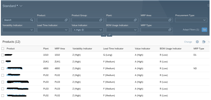
Figure 5: Lead Time Classification App
It will show you the classifications of products based on the threshold parameters for good issue values, variability coefficient, BOM usage and decoupled lead time as discussed above. You can use available filters on them to get a clear picture on critical materials.
Based the Variability (XYZ) and Lead time (EFG) classifications results, you may need to fine tune the values for Variability Factor and Lead time factor that you have maintained in your Buffer Profile configuration (Table: PPH_BF_PRFLDET_V), until DDMRP reaches certain maturity level to give desired results.
Along with Buffer Profile configuration, there is another import factor that we need to consider is – the qualified order spikes or the spiked in demand. The purpose to consider them is to protect your buffer inventory from irregularities in future consumption which was not taken into account, considering the current Lead time and Variability factors as seen above. However, I will cover this topic in an upcoming blog.
So, to conclude – I have tried to shed some light on - the Buffer Profiles configuration in SAP S/4HANA DDMRP, the concept behind Buffer Zones and how Buffer Profiles work in tandem with Product and Lead time classification tools.
Thanks for reading! Appreciate your feedback and comments.
5 Comments
You must be a registered user to add a comment. If you've already registered, sign in. Otherwise, register and sign in.
Labels in this area
-
"mm02"
1 -
A_PurchaseOrderItem additional fields
1 -
ABAP
1 -
ABAP Extensibility
1 -
ACCOSTRATE
1 -
ACDOCP
1 -
Adding your country in SPRO - Project Administration
1 -
Advance Return Management
1 -
AI and RPA in SAP Upgrades
1 -
Approval Workflows
1 -
ARM
1 -
ASN
1 -
Asset Management
1 -
Associations in CDS Views
1 -
auditlog
1 -
Authorization
1 -
Availability date
1 -
Azure Center for SAP Solutions
1 -
AzureSentinel
2 -
Bank
1 -
BAPI_SALESORDER_CREATEFROMDAT2
1 -
BRF+
1 -
BRFPLUS
1 -
Bundled Cloud Services
1 -
business participation
1 -
Business Processes
1 -
CAPM
1 -
Carbon
1 -
Cental Finance
1 -
CFIN
1 -
CFIN Document Splitting
1 -
Cloud ALM
1 -
Cloud Integration
1 -
condition contract management
1 -
Connection - The default connection string cannot be used.
1 -
Custom Table Creation
1 -
Customer Screen in Production Order
1 -
Data Quality Management
1 -
Date required
1 -
Decisions
1 -
desafios4hana
1 -
Developing with SAP Integration Suite
1 -
Direct Outbound Delivery
1 -
DMOVE2S4
1 -
EAM
1 -
EDI
2 -
EDI 850
1 -
EDI 856
1 -
edocument
1 -
EHS Product Structure
1 -
Emergency Access Management
1 -
Energy
1 -
EPC
1 -
Financial Operations
1 -
Find
1 -
FINSSKF
1 -
Fiori
1 -
Flexible Workflow
1 -
Gas
1 -
Gen AI enabled SAP Upgrades
1 -
General
1 -
generate_xlsx_file
1 -
Getting Started
1 -
HomogeneousDMO
1 -
IDOC
2 -
Integration
1 -
learning content
2 -
LogicApps
2 -
low touchproject
1 -
Maintenance
1 -
management
1 -
Material creation
1 -
Material Management
1 -
MD04
1 -
MD61
1 -
methodology
1 -
Microsoft
2 -
MicrosoftSentinel
2 -
Migration
1 -
MRP
1 -
MS Teams
2 -
MT940
1 -
Newcomer
1 -
Notifications
1 -
Oil
1 -
open connectors
1 -
Order Change Log
1 -
ORDERS
2 -
OSS Note 390635
1 -
outbound delivery
1 -
outsourcing
1 -
PCE
1 -
Permit to Work
1 -
PIR Consumption Mode
1 -
PIR's
1 -
PIRs
1 -
PIRs Consumption
1 -
PIRs Reduction
1 -
Plan Independent Requirement
1 -
Premium Plus
1 -
pricing
1 -
Primavera P6
1 -
Process Excellence
1 -
Process Management
1 -
Process Order Change Log
1 -
Process purchase requisitions
1 -
Product Information
1 -
Production Order Change Log
1 -
Purchase requisition
1 -
Purchasing Lead Time
1 -
Redwood for SAP Job execution Setup
1 -
RISE with SAP
1 -
RisewithSAP
1 -
Rizing
1 -
S4 Cost Center Planning
1 -
S4 HANA
1 -
S4HANA
3 -
Sales and Distribution
1 -
Sales Commission
1 -
sales order
1 -
SAP
2 -
SAP Best Practices
1 -
SAP Build
1 -
SAP Build apps
1 -
SAP Cloud ALM
1 -
SAP Data Quality Management
1 -
SAP Maintenance resource scheduling
2 -
SAP Note 390635
1 -
SAP S4HANA
2 -
SAP S4HANA Cloud private edition
1 -
SAP Upgrade Automation
1 -
SAP WCM
1 -
SAP Work Clearance Management
1 -
Schedule Agreement
1 -
SDM
1 -
security
2 -
Settlement Management
1 -
soar
2 -
SSIS
1 -
SU01
1 -
SUM2.0SP17
1 -
SUMDMO
1 -
Teams
2 -
User Administration
1 -
User Participation
1 -
Utilities
1 -
va01
1 -
vendor
1 -
vl01n
1 -
vl02n
1 -
WCM
1 -
X12 850
1 -
xlsx_file_abap
1 -
YTD|MTD|QTD in CDs views using Date Function
1
- « Previous
- Next »
Related Content
- SAP GTS classification not recorded at compliance document creation in Enterprise Resource Planning Q&A
- Posting Journal Entries with Tax Using SOAP Posting APIs in Enterprise Resource Planning Blogs by SAP
- Quick Start guide for PLM system integration 3.0 Implementation/Installation in Enterprise Resource Planning Blogs by SAP
- Futuristic Aerospace or Defense BTP Data Mesh Layer using Collibra, Next Labs ABAC/DAM, IAG and GRC in Enterprise Resource Planning Blogs by Members
- Service with Advanced Execution and Resource-related Billing in Enterprise Resource Planning Blogs by SAP
Top kudoed authors
| User | Count |
|---|---|
| 2 | |
| 2 | |
| 2 | |
| 2 | |
| 2 | |
| 2 | |
| 2 | |
| 2 | |
| 1 | |
| 1 |