
- SAP Community
- Products and Technology
- Technology
- Technology Blogs by SAP
- Open Source GIS with SAP HANA
Technology Blogs by SAP
Learn how to extend and personalize SAP applications. Follow the SAP technology blog for insights into SAP BTP, ABAP, SAP Analytics Cloud, SAP HANA, and more.
Turn on suggestions
Auto-suggest helps you quickly narrow down your search results by suggesting possible matches as you type.
Showing results for
Product and Topic Expert
Options
- Subscribe to RSS Feed
- Mark as New
- Mark as Read
- Bookmark
- Subscribe
- Printer Friendly Page
- Report Inappropriate Content
11-26-2019
5:58 PM
 QGIS, GeoServer & more: SAP HANA Spatial ❤️ Integration
Introduction
SAP’s in-memory database SAP HANA features a geospatial engine, which makes SAP HANA a predestinated storage for geospatial vector data. Once data is residing in SAP HANA developers can leverage the power of HANA’s multi-model engines (e.g. graph and json document store) as well as the advanced analytics capabilities and embedded machine learning (e.g. PAL, APL, EML).
Learn more about SAP HANA’s multi-model capabilities.
Furthermore, with the release of HANA2 SP04 there have some advances been made in the area of spatial analytics. The most prominent feature being the in-database hexagonal clustering.
Entertaining resource to learn more about Hexagonal Tessellation.
However, even the most sophisticated spatial analytics model, which already adds value by running as a backend component, deserves to be presented adequately instead of being solely “in-database”. At SAP we offer solutions such as SAP Analytics Cloud which feature map visualizations for business users. GIS (Geographic Information System) departments and developers do require a much broader GIS specific feature set. For that reason, SAP has a strong partnership with Esri, the market leader for commercial GIS software. The spatial component of SAP HANA is designed to seamlessly integrate with Esri ArcGIS and serves as certified geodatabase for Esri customers.
Learn more about Esri and SAP HANA as geodatabase.
Complementary to proprietary GIS software many customers run hybrid landscapes with Open Source GIS solutions like QGIS. In this article we will describe how to connect SAP HANA with the QGIS desktop client using GeoServer.
Learn more about QGIS and GeoServer.
Technically we will setup the whole stack on a local laptop. All necessary software components – including SAP HANA Express – can be downloaded free of charge.
This guide focuses on an end-to-end scenario and highlights the major building blocks of the setup. For detailed technical instructions we will link other articles. However, if you follow the straight path you should be able to do the whole setup in less than 30 minutes (excluding download times).
Have fun while getting your hands dirty!
Summary
In this tutorial you will learn how to
- Install SAP HANA Express, GeoServer and QGIS
- Setup the integration between the components
- Upload a spatial dataset to SAP HANA
- Expose a plain table via GeoServer
- Expose a derived view via GeoServer
- Visualize the result in QGIS
 SAP HANA Spatial seamlessly integrates GIS and Business data
If you are interested in further resources on SAP HANA Spatial and the integration of Esri ArcGIS please review the following blog, which gathers the most important tutorials and articles:
https://blogs.sap.com/2017/11/15/sap-hana-spatial-resources/
Installing required software
Everything you need for this tutorial is downloadable at no license cost and can be installed on a laptop with sufficient memory. Please find the individual components in the table below:
| SAP HANA Express | For this tutorial you can use any SAP HANA instance that you may already have running. Just make sure that you use at least HANA2 SP4 – otherwise Hexagonal Clustering will not be available. If you do not have an instance available the quickest solution is to download and install SAP HANA Express. http://www.sap.com/sap-hana-express The installer will come with detailed instructions on the initial setup. A plain vanilla system is sufficient as the spatial component is contained out of the box. Version used here: SAP HANA Express 2.0 SPS04 |
| GeoServer | Next you will need to download and setup GeoServer. http://geoserver.org/download/ Just unpack the downloaded content and move it to a directory of your preference. There is no installation required. Before you can actually start the GeoServer, you will need to install the SAP HANA Plugin into GeoServer. Version used here: GeoServer 2.16.0 |
| HANA Plug-in for GeoServer | In the GeoServer Documentation you will find a step-by-step guide how to enable support for SAP HANA in GeoServer: https://docs.geoserver.org/latest/en/user/community/hana/index.html Version used here: SAP HANA DataStore 22.0 (corresponds to GeoServer 2.16.0) |
| QGIS | Last but not least we are going to need an installation of QGIS. The latest installer can be found on the QGIS site. Just do the default installation – nothing particular to consider here. https://www.qgis.org/ Version used here: QGIS 3.10.0 |
Happy installing!
Uploading Sample Data to SAP HANA
Of course, if you already have you favorite geospatial dataset in your HANA instance, you can skip this step. Just make sure to have it stored in an ST_Geometry column.
If you are looking for a nice dataset to play around with, I recommend the data that AirBnB has released under a Creative Commons license. For our example we are going to use the Summary File of Berlin, which can be obtained from the following URL:
http://insideairbnb.com/get-the-data.html
Upload CSV File
There are multiple ways of uploading this CSV content into SAP HANA. I would like to briefly mention two:
- You may use the built-in import statement:
https://help.sap.com/viewer/4fe29514fd584807ac9f2a04f6754767/2.0.04/en-US/20f712e175191014907393741f... - If you are using Python, there is a very neat way by leveraging Pandas and SQLAlchemy. To follow this path, you first need to setup the HANA plugin for SQLAlchemy:
https://github.com/SAP/sqlalchemy-hana/
Afterwards you can download the data via Pandas:
df_download = pd.read_csv('http://data.insideairbnb.com/germany/be/berlin/2019-09-19/visualisations/listings.csv')
And persist it in HANA:
hdb_connection = sqlalchemy.create_engine('hana://%s:%s@%s:%s' % (hdb_user, hdb_password, hdb_host, hdb_port)).connect()

df_download.to_sql(name = 'listings_airbnb_berlin', con = hdb_connection, if_exists = 'replace')
Adjust Table Structure
Now that you have the plain data in HANA, we still need maintain the primary key and construct a geometry column out of the latitude and longitude values. Eventually you could use any of the more than 4000 Spatial Reference Systems from EPSG that SAP HANA supports. However, since we deal with data from Berlin it is a good idea to use a local SRS, which in this case would be e.g. Gauss-Kruger (EPSG 31468).
We can install 31468 by executing the following statement on a SQL console:
CREATE SPATIAL REFERENCE SYSTEM "DHDN / 3-degree Gauss-Kruger zone 4" IDENTIFIED BY 31468 DEFINITION 'PROJCS["DHDN / 3-degree Gauss-Kruger zone 4",GEOGCS["DHDN",DATUM["Deutsches_Hauptdreiecksnetz",SPHEROID["Bessel 1841",6377397.155,299.1528128,AUTHORITY["EPSG","7004"]],TOWGS84[598.1,73.7,418.2,0.202,0.045,-2.455,6.7],AUTHORITY["EPSG","6314"]],PRIMEM["Greenwich",0,AUTHORITY["EPSG","8901"]],UNIT["degree",0.0174532925199433,AUTHORITY["EPSG","9122"]],AUTHORITY["EPSG","4314"]],PROJECTION["Transverse_Mercator"],PARAMETER["latitude_of_origin",0],PARAMETER["central_meridian",12],PARAMETER["scale_factor",1],PARAMETER["false_easting",4500000],PARAMETER["false_northing",0],UNIT["metre",1,AUTHORITY["EPSG","9001"]],AUTHORITY["EPSG","31468"]]' ORGANIZATION "EPSG" IDENTIFIED BY 31468 TRANSFORM DEFINITION '+proj=tmerc +lat_0=0 +lon_0=12 +k=1 +x_0=4500000 +y_0=0 +ellps=bessel +towgs84=598.1,73.7,418.2,0.202,0.045,-2.455,6.7 +units=m +no_defs ' TYPE PLANAR COORDINATE X BETWEEN 4386858.108907308 AND 4597711.685158775 COORDINATE Y BETWEEN 5251253.290839581 AND 6052196.769576701 TOLERANCE DEFAULT SNAP TO GRID DEFAULT POLYGON FORMAT 'EvenOdd' STORAGE FORMAT 'Internal';Full list of creation statements for Spatial Reference Systems
After having 31468 handy, we can run these both statements to append a column of type ST_GEOMETRY and fill it with geometries derived from the given latitude and longitude values:
ALTER TABLE LISTINGS_AIRBNB_BERLIN ADD (SHAPE ST_GEOMETRY(31468))

UPDATE LISTINGS_AIRBNB_BERLIN SET SHAPE = ST_GEOMFROMTEXT('Point('||LONGITUDE||' '||LATITUDE||')', 4326).ST_TRANSFORM(31468)
Finally, we need to add a primary key constraint to the already existing ID column. This will be required by GeoServer later on to publish the WFS service.
ALTER TABLE LISTINGS_AIRBNB_BERLIN ADD PRIMARY KEY (ID)Full Code Snippet
Given that you installed SRS 31468, the full process of uploading and converting data can be achieved with the following Python script:
import sqlalchemy

import pandas as pd


df_download = pd.read_csv('http://data.insideairbnb.com/germany/be/berlin/2019-09-19/visualisations/listings.csv')

hdb_connection = sqlalchemy.create_engine('hana://%s:%s@%s:%s' % (hdb_user, hdb_password, hdb_host, hdb_port)).connect()

df_download.to_sql(name = 'listings_airbnb_berlin', con = hdb_connection, if_exists = 'replace')


hdb_connection.execute("ALTER TABLE LISTINGS_AIRBNB_BERLIN ADD (SHAPE ST_GEOMETRY(31468))")

hdb_connection.execute("UPDATE LISTINGS_AIRBNB_BERLIN SET SHAPE = ST_GEOMFROMTEXT('Point('||LONGITUDE||' '||LATITUDE||')', 4326).ST_TRANSFORM(31468)")


hdb_connection.execute("ALTER TABLE LISTINGS_AIRBNB_BERLIN ADD PRIMARY KEY (ID)")
Congratulations! There is now some spatial data waiting for you in SAP HANA!
Exposing Data via GeoServer
We want to use GeoServer in order to populate the data in a way, that QGIS can understand. Most commonly we would use a Web Feature Service (WFS) for this. We can use WFS to expose both datasets – the original point data as well as the view containing hexagonal cells and density information.
Run GeoServer by using one of the platform-dependend startup scripts in the bin directory or by calling
java -jar start.jarin the GeoServer directory. Once the server has started the admin UI in the default installation will be reachable via
http://localhost:8080/geoserver
The default username/password is admin/geoserver.
GeoServer is now up and running!
Exposing Data from a HANA Table
We will need to create a Workspace, Store and two Layers in GeoServer. What we want to achieve is that one layer exposes the original point data whereas the second layer exposes some processed data (i.e. the hexagonal clustering).
Create a workspace by selecting the entry "Workspace" on the left sidebar and then click "Add new Workspace"

Create a store by selecting "Stores" on the left sidebar and then click "Add new Store". On the following page select the SAP HANA Plugin.

Fill in the connection details and leave the enhanced parameters with the default values. It is also a good idea to explicitly name the schema you are working in - although this is not a mandatory field. GeoServer may otherwise be mislead if the same table is existent in more than one schema.

Publish the layer by selecting your table from the list of spatial objects and click "Publish".

In the following screen you will have to verify that
- the right SRS has been chosen by GeoServer. You need to correct the SRS in case it is incorrect (i.e. it is not 31468 for our example).
- the bounding boxes have been calculated. You can achieve this by computing the bounding boxes from the given data.

After saving the new layer your list of layers should contain a new entry. You have created your first service to expose your raw point data via GeoServer!

Exposing Data as a View
So now we want to do some basic analytics to gain some more insights from our dataset. We will build a view on our dataset, which does a hexagonal clustering and aggregates the number of listings per cluster. This can be used to visualize something similar to a heatmap.
We again add a new layer by choosing "Layers" from the left menu bar and then click "Add a new layer". However, this time we will choose to "Configure a new SQL view".

In the following screen we provide a layer name of our choice and insert the following SQL Statement:
SELECT

   ST_ClusterID() as clusterid,

   ST_ClusterCell() as clustercell,

   COUNT(*) as n_listings

FROM LISTINGS_AIRBNB_BERLIN

GROUP CLUSTER BY shape USING HEXAGON X CELLS 50
Make sure that you
- refresh the attribute list to show the output columns of the select statement
- choose an appropriate identifier column
- choose the right type and SRID for the geometry column
The following screen is similar to the one when creating a new layer from a plain table. Again, check the SRID and the bounding boxes (see description above).
Superb! We exposed the point data as well as the hexagonal clustering as a WFS service. We can reward ourselves by looking at the preview of the shapes from within GeoServer.
You can access the preview by selecting the "Layer Preview" on the left side bar and then selecting the "OpenLayers" format of the respective layer.

Eventually you will see the respective layers in the browser. You can even click individual geometries to retrieve further line item information (e.g. the number of listings per cell)!
- Raw Point Data - LISTINGS_AIRBNB_BERLIN

- Hexagonal Cells - LISTINGS_AIRBNB_BERLIN_CLUSTER

Consuming WFS Service in QGIS
We have already seen a visualization of our geometries. Now we will load the data into QGIS and build a visualization which actually gives us some more insights on the vast amount of listing data.
The base URL for WFS (OWS) service is composed out of the workspace name, which in our case is "AirBnB":
http://localhost:8080/geoserver/AirBnB/ows
To configure that service in QGIS, we open up the client and right-click "WFS" in the left side bar to add a new connection.

In the following dialog we paste the URL for our service (as mentioned above) and give it a meaningful name. The remaining configuration can be left on standard values.

After adding the service you should be able to see both of your layer in the QGIS tree. Furthermore, you should see an OpenStreetMap layer in the tree below "XYZ Tiles".
Add the OpenStreetMap layer by double-clicking the layer name. Afterwards double-click the clustering layer (LISTINGS_AIRBNB_BERLIN_CLUSTERING. You will see your hexagonal clusters which are generate by a view on SAP HANA on the map. Make sure that the sorting of layers is correct in the lower right window - otherwise the map layer may be hiding your hexagonal cells.

Well, next step is that we would like to color the hexagons based on the number of listings within the cell. Remember that this is an attribute which we have calculated in our view and which is also transferred to QGIS via the WFS service.
For setting up the appearance of the cluster layer, you need to right click the layer in the lower left corner and choose "Properties". In the properties dialog, select the "Symbology" tab.
Change the style from "Single Symbol" to "Graduated" and choose the attribute field "N_LISTINGS" as value. Click on "Classify" to generate an initial coloring scale.

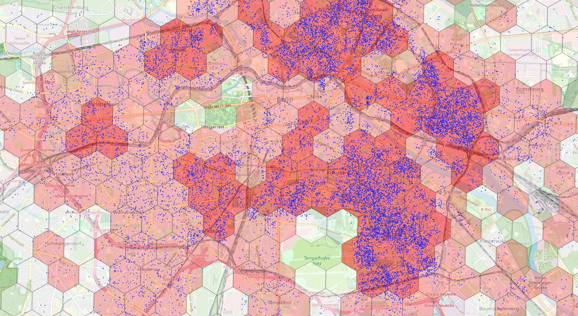
To make the result look a bit nicer you can play around with the different visualization styles. I chose a logarithmic scale and set an opacity of 50% for the layer. This way you can see the map shine through your polygons.

As opposed to seeing > 20k points on a map we are now able to easily spot the neighbourhoods of Berlin with the most AirBnB offerings. To compare the highlighting of the cells with the raw point data, we can now add another layer with raw points and set the point size to the minimum available value, which can be done again from the "Symbology" tab in "Properties".
We can now move and zoom on the map to analyze the distribution of AirBnB listings.
By selecting the "Identify Features" tool from the tool bar, we are able to retrieve the full line item from SAP HANA for the object that we select on the map.


If you made it up until here and see something similar on your screen, you have successfully unlocked the world of spatial analytics on your machine! I am looking forward reading your blog posts on integrating HANA Spatial into business processes and infusing the spatial dimension into your machine learning models!
Thanks for reading, Spatial Enthusiast!
- SAP Managed Tags:
- Open Source,
- SAP HANA,
- SAP HANA, express edition,
- SAP HANA multi-model processing,
- SAP HANA Spatial
Labels:
21 Comments
You must be a registered user to add a comment. If you've already registered, sign in. Otherwise, register and sign in.
Labels in this area
-
ABAP CDS Views - CDC (Change Data Capture)
2 -
AI
1 -
Analyze Workload Data
1 -
BTP
1 -
Business and IT Integration
2 -
Business application stu
1 -
Business Technology Platform
1 -
Business Trends
1,658 -
Business Trends
91 -
CAP
1 -
cf
1 -
Cloud Foundry
1 -
Confluent
1 -
Customer COE Basics and Fundamentals
1 -
Customer COE Latest and Greatest
3 -
Customer Data Browser app
1 -
Data Analysis Tool
1 -
data migration
1 -
data transfer
1 -
Datasphere
2 -
Event Information
1,400 -
Event Information
66 -
Expert
1 -
Expert Insights
177 -
Expert Insights
293 -
General
1 -
Google cloud
1 -
Google Next'24
1 -
Kafka
1 -
Life at SAP
780 -
Life at SAP
13 -
Migrate your Data App
1 -
MTA
1 -
Network Performance Analysis
1 -
NodeJS
1 -
PDF
1 -
POC
1 -
Product Updates
4,577 -
Product Updates
340 -
Replication Flow
1 -
RisewithSAP
1 -
SAP BTP
1 -
SAP BTP Cloud Foundry
1 -
SAP Cloud ALM
1 -
SAP Cloud Application Programming Model
1 -
SAP Datasphere
2 -
SAP S4HANA Cloud
1 -
SAP S4HANA Migration Cockpit
1 -
Technology Updates
6,873 -
Technology Updates
417 -
Workload Fluctuations
1
Related Content
- What is the difference between OMS and OMM, while using SAP Commerce with S/4 Hana which to use? in Technology Q&A
- App to automatically configure a new ABAP Developer System in Technology Blogs by Members
- Data Privacy Embedding Model via Core AI in Technology Q&A
- From R/3 4.7 to ECC 6.0 EHP 7/8 in Technology Q&A
- Onboarding Users in SAP Quality Issue Resolution in Technology Blogs by SAP
Top kudoed authors
| User | Count |
|---|---|
| 35 | |
| 25 | |
| 13 | |
| 7 | |
| 7 | |
| 6 | |
| 6 | |
| 6 | |
| 5 | |
| 4 |