
- SAP Community
- Products and Technology
- Technology
- Technology Blogs by SAP
- SAP Data Intelligence : Advanced Attrition Data Sc...
Technology Blogs by SAP
Learn how to extend and personalize SAP applications. Follow the SAP technology blog for insights into SAP BTP, ABAP, SAP Analytics Cloud, SAP HANA, and more.
Turn on suggestions
Auto-suggest helps you quickly narrow down your search results by suggesting possible matches as you type.
Showing results for
Advisor
Options
- Subscribe to RSS Feed
- Mark as New
- Mark as Read
- Bookmark
- Subscribe
- Printer Friendly Page
- Report Inappropriate Content
11-19-2019
1:33 AM
In this video I'll be showing the full process to create a logistic regression model developed in Python inside SAP Data Intelligence using a training set of employee attrition. This model will then be exposed thru an REST-API using SAP Data Intelligence. To create this demo I've used this great blog from Andreas Forster, a great part of this blog is directly copied from his work, with his permission. If at any point you find yourself lost in my demo, please refer back to Andreas' blog and follow his steps through. He goes much more in detail with what to do and explains every component in a much more detailed manner.
Please note that the data used here is fake and contains no real information.
Dataset and business question
Our dataset is a small CSV file, which contains 2800 fake employee information with 64 columns of various information and also with a column indicating, job title, several competencies, salary, etc...
| ID | Country | DOB | AgeJoined | Age | YearsOfService | ... |
| 1 | France | 03/04/1992 | 27 | 27 | 0 | |
| 2 | France | 13/09/1984 | 33 | 35 | 2 | |
| 3 | France | 21/02/1981 | 38 | 38 | 0 | |
| 4 | France | 15/09/1967 | 27 | 52 | 25 | |
| 5 | France | 11/02/1994 | 21 | 25 | 4 |
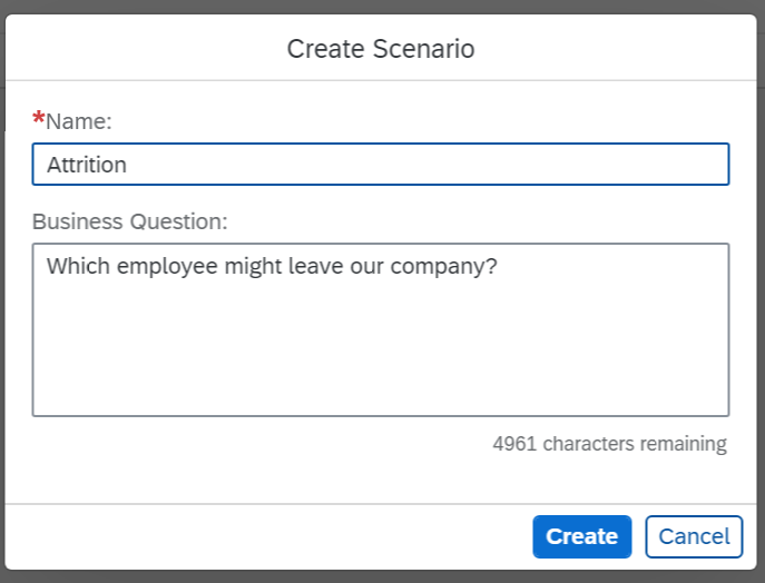
The business question we are trying to answer here is the risk of attrition of an employee. In our dataset, we have a column LEFT saying if the employee has left the company of not. We will use this column for training/testing purpose and then try to run it for our existing or new employees to identify those who might leave us.
In this demo I'm loading this dataset in min.io to simulate an Amazon S3 bucket. I have also loaded this dataset in my own SAP HANA database to develop my python code in the SAP Data Intelligence provided Jupyter Lab Notebook.
Data connection
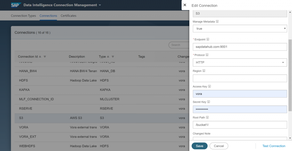
First we need to define all the connections that we will be using:
We need to configure our S3 bucket connection and have it point to our bucket. You can verify the connection by clicking on Test Connection.
ML Scenario
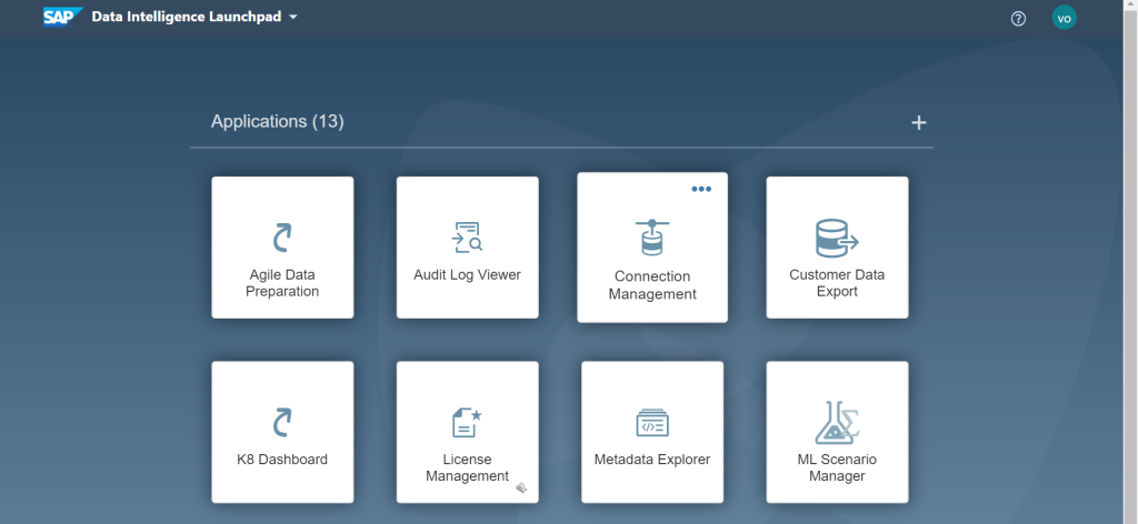
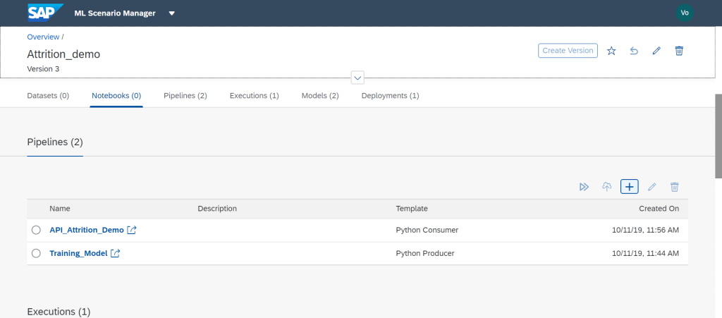
After we have loaded our file, we can start working on the actual Data Science part of our task. Go back to the main page of SAP Data Intelligence and click into the “ML Scenario Manager”.
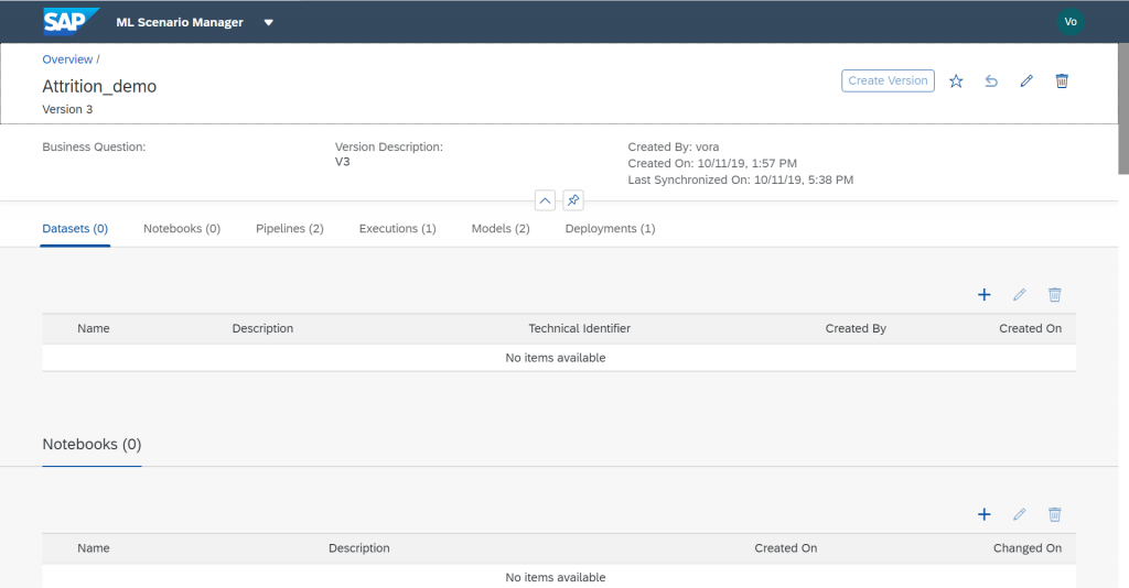
I will not go into the details of the machine learning python script here but basically this is where I created the notebook to perform my analysis. We will also create two pipelines here, one to perform the training of our model and the second one to deploy our REST-API using this same model.
Logistic Regression model training
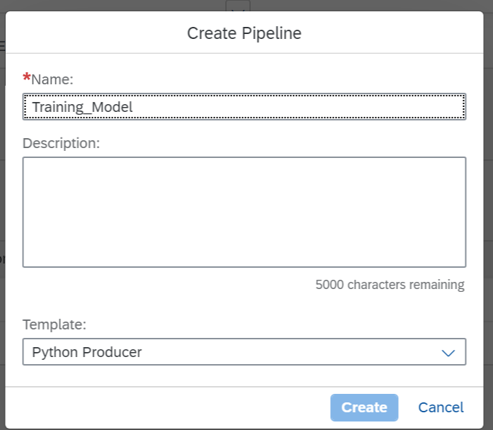
First we will create a Training Pipeline by clicking the "+" sign in the Notebooks section.
For this I will use the Python Producer template
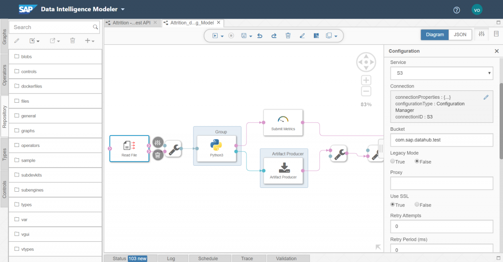
We then need to configure the read file component of our pipeline and have it point to our previously defined S3 bucket.
Then we simply need to enter the path to our csv file in the bucket.
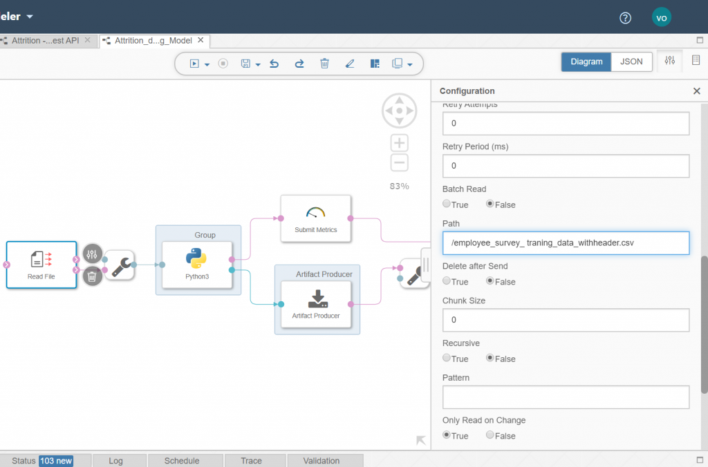
We then need to enter our python code in the Python3 component.
Here is the code that was used in my component:
import sklearn

from sklearn.model_selection import train_test_split

from sklearn import preprocessing

from sklearn.linear_model import LogisticRegression

import pandas as pd

from sklearn import metrics

import io

import numpy as np


# Example Python script to perform training on input data & generate Metrics & Model Blob

def on_input(data):


    # Obtain data

    df_data = pd.read_csv(io.StringIO(data), sep=";")

    # Creating labelEncoder

    le = preprocessing.LabelEncoder()

    # Categorical features to numerical features

    df_data['Gender']=le.fit_transform(df_data['Gender'])

    df_data['JobType']=le.fit_transform(df_data['JobType'])

    df_data['BirthCountry']=le.fit_transform(df_data['BirthCountry'])

    # Balancing the dataset

    Left = df_data[df_data["LEFT"]==1].sample(200)

    Stayed = df_data[df_data["LEFT"]==0].sample(200)

    balanced_df = pd.concat([Left, Stayed],ignore_index=False, sort=False)

    # Normalization

    column_names_to_normalize = ['Age_Years', 'Salary','VerbalCommunication','Teamwork',

           'CommercialAwareness','AnalysingInvestigating','InitiativeSelfMotivation','Drive','WrittenCommunication',

           'Flexibility','TimeManagement','PlanningOrganising','DaysSickYTD','ContractedHoursperWeek','PerformanceGrade2015',

           'DaysWithoutRaise','Gender','JobType']

    X = balanced_df[['Age_Years', 'Salary','VerbalCommunication','Teamwork',

           'CommercialAwareness','AnalysingInvestigating','InitiativeSelfMotivation','Drive','WrittenCommunication',

           'Flexibility','TimeManagement','PlanningOrganising','DaysSickYTD','ContractedHoursperWeek','PerformanceGrade2015',

           'DaysWithoutRaise','Gender','JobType']]

    # We will be using a min max scaler for normalization

    min_max_scaler = preprocessing.MinMaxScaler()

    df = X

    x = df[column_names_to_normalize].values

    x_scaled = min_max_scaler.fit_transform(x)

    df_temp = pd.DataFrame(x_scaled, columns=column_names_to_normalize, index = df.index)

    df[column_names_to_normalize] = df_temp

    X = df_temp

    # Converting string labels into numbers.

    y=le.fit_transform(balanced_df['LEFT'])

    #  Slicing dataset between train and test

    X_train, X_test, y_train, y_test = train_test_split(X, y, test_size=0.2, random_state=0)

    # Training the Model

    clf= LogisticRegression(verbose = 3)

    clf_trained = clf.fit(X_train, y_train)

    y_pred = clf_trained.predict(X_test)


    MeanAbsoluteError=metrics.mean_absolute_error(y_test, y_pred)

    MeanSquaredError=metrics.mean_squared_error(y_test, y_pred)

    RootMeanSquaredError=np.sqrt(metrics.mean_squared_error(y_test, y_pred))


    # to send metrics to the Submit Metrics operator, create a Python dictionary of key-value pairs

    metrics_dict = {"Mean Absolute Error": str(MeanAbsoluteError),"Mean Squared Error": str(MeanSquaredError), "Root Mean Squared Error": str(RootMeanSquaredError), "n": str(len(df_data))}


    # send the metrics to the output port - Submit Metrics operator will use this to persist the metrics

    api.send("metrics", api.Message(metrics_dict))


    # create & send the model blob to the output port - Artifact Producer operator will use this to persist the model and create an artifact ID

    import pickle

    model_blob = pickle.dumps(clf_trained)

    api.send("modelBlob", model_blob)


api.set_port_callback("input", on_input)
Exit the code, save the pipeline and we now can train the model. Go back to the ML Scenario page and select your newly created pipeline.
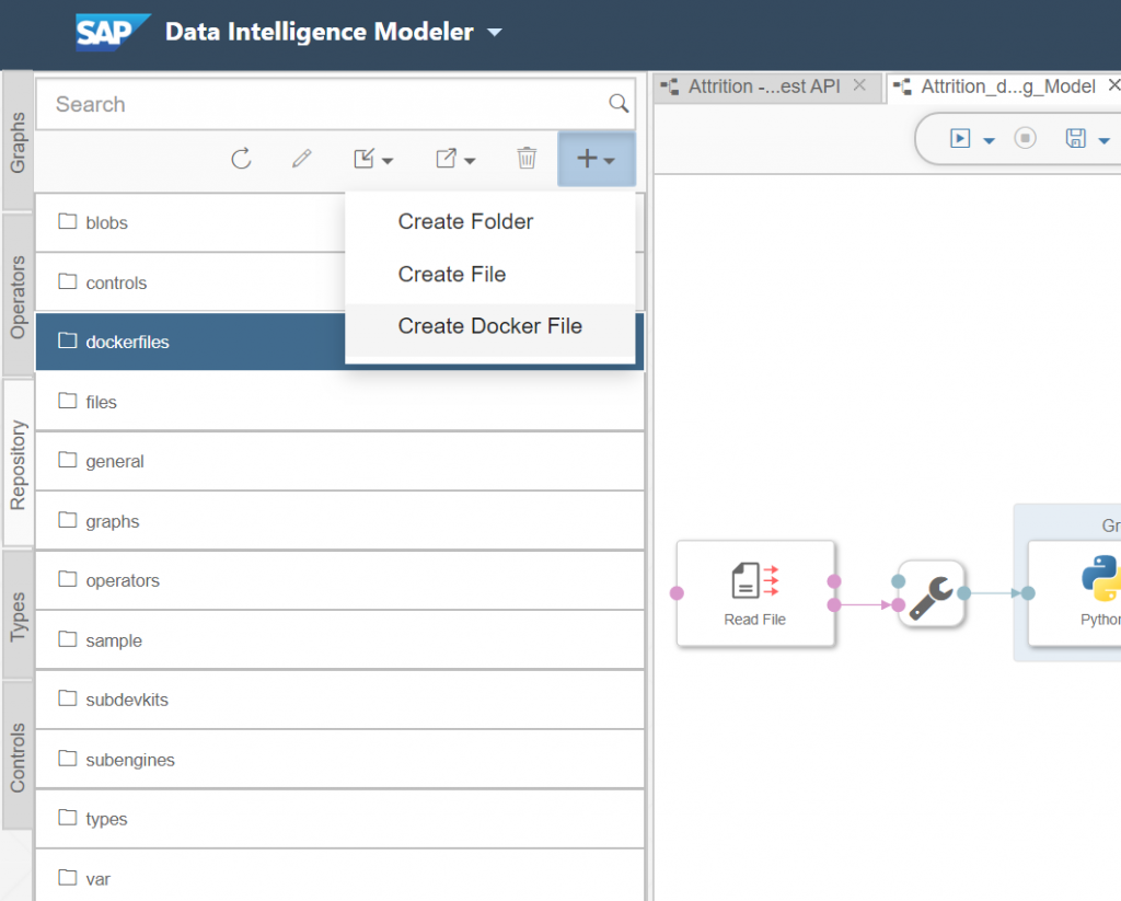
One very important step here is to define the docker image for our Python3 component. This will allow us to use specific libraries for this pipeline without impacting others. Go to repository on the left side of SAP Data Intelligence and "Create a Docker File".
FROM $com.sap.opensuse.python36

RUN python3.6 -m pip install numpy==1.16.4

RUN python3.6 -m pip install pandas==0.24.0

RUN python3.6 -m pip install sklearn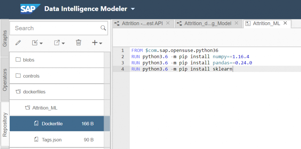
After you have done that you can enter specific tags to use with our Python component. Click on the configuration panel and enter the following information.
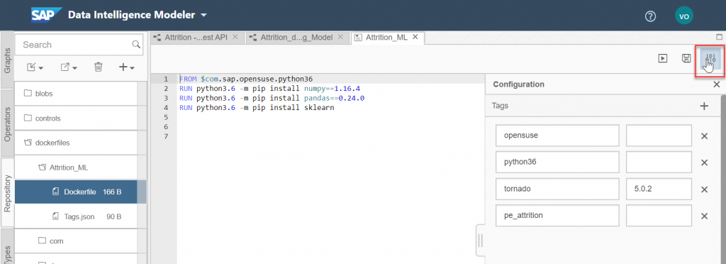
"opensuse", "python36" and "tornado". For "tornado" also enter the version "5.0.2". We also need to enter a specific tag for this dockerfile. I've used "pe_attrition".
Now save the Docker file and click the “Build” icon to start building the Docker image.
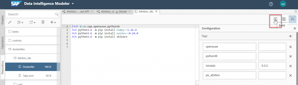
Wait until the build is successful. You can know use this docker file for your Python component.
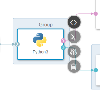
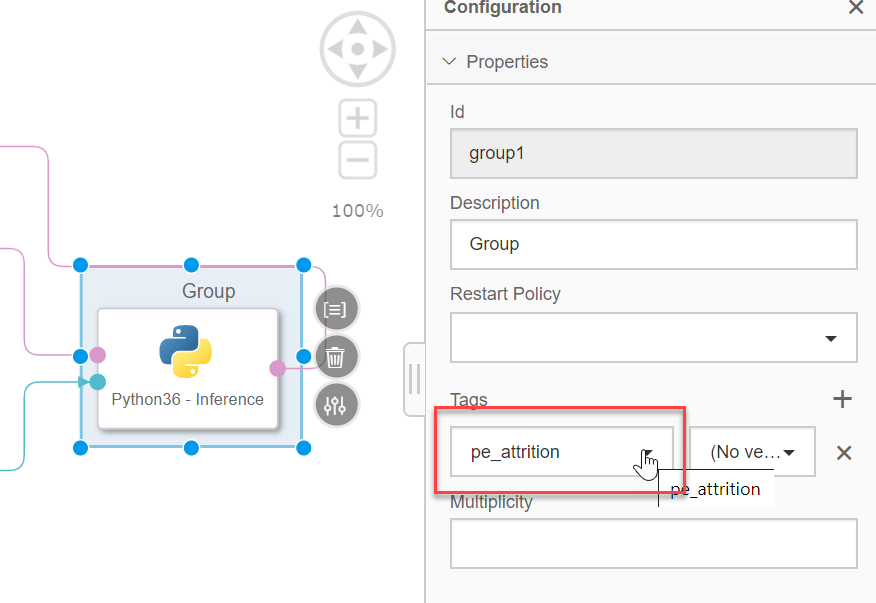
To do so, we go back to the graphical pipeline and right click the Python3 component and select "Group".

In the tags, we will add the previously created tag, "pe_attrition".
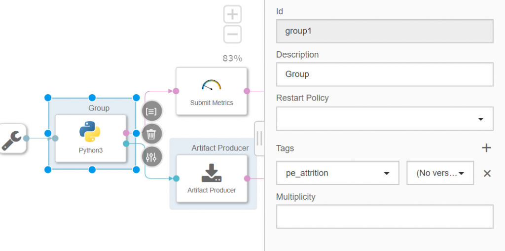
You can now save the graph.
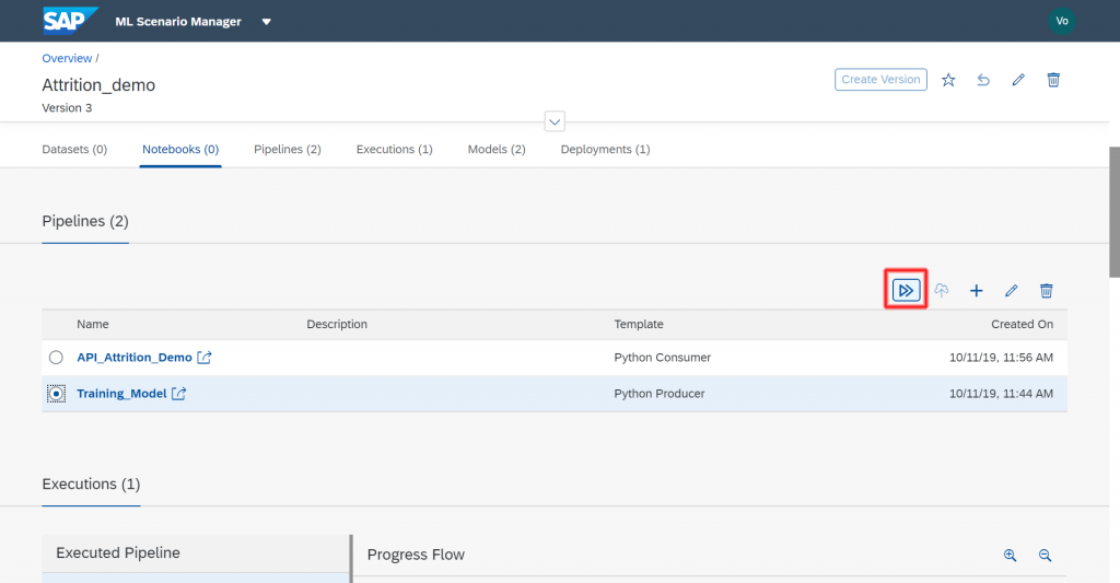
The pipeline is now complete and we can run it. Go back to the ML Scenario, select your pipeline and execute it.
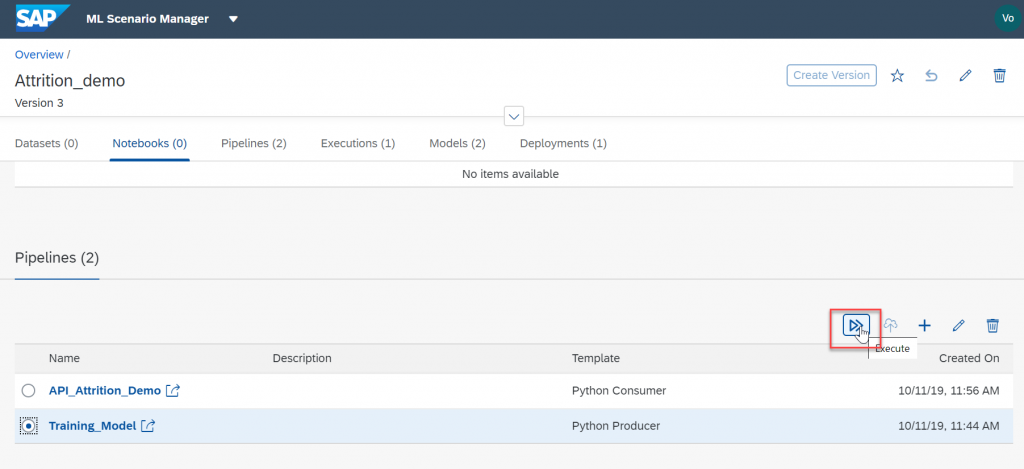
Click thru all the steps and give your model a name. Wait till the model is executed.
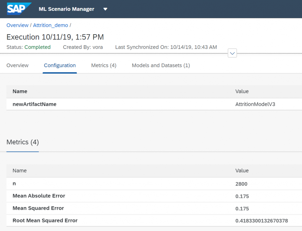
You can now look at the results of our model thru the metrics that we used in our python code.
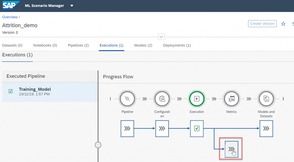
If the results of our metrics are good enough we can proceed with deploying the model as a REST API.
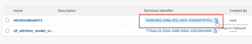
Go back to your ML scenario and copy the model technical identifier
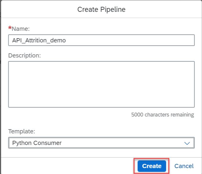
Pushing the model as a REST-API
Let's create a second pipeline. For this we will be using a Python Consumer template.
We only need to change the Submit Artifact Name component "Content" value and change it to ${modelTechnicalIdentifier}. As explained in Andreas' blog, this change will enable us to pass the model’s technical identifier to the pipeline.
I then modified the code in the Python3 component to the following :
import json

import pickle

from sklearn import preprocessing

import pandas as pd


# Global vars to keep track of model status

model = None

model_ready = False


# Validate input data is JSON

def is_json(data):

  try:

    json_object = json.loads(data)

  except ValueError as e:

    return False

  return True


# When Model Blob reaches the input port

def on_model(model_blob):

    global model

    global model_ready


    model = pickle.loads(model_blob)

    model_ready = True

    api.logger.info("Model Received & Ready")


# Client POST request received

def on_input(msg):

    error_message = ""

    success = False

    prediction = None

    df_data = None


    try:

        api.logger.info("POST request received from Client - checking if model is ready")

        if model_ready:

            api.logger.info("Model Ready")

            api.logger.info("Received data from client - validating json input")


            user_data = msg.body.decode('utf-8')

            # Received message from client, verify json data is valid

            if is_json(user_data):

                api.logger.info("Received valid json data from client - ready to use")


                # apply your model

                # Obtain data

                data = json.loads(user_data)

                df_data = pd.DataFrame(data, index=[0])

                # Creating labelEncoder

                le = preprocessing.LabelEncoder()

                # Categorical features to numerical features

                df_data['Gender']=le.fit_transform(df_data['Gender'])

                df_data['JobType']=le.fit_transform(df_data['JobType'])

                df_data['BirthCountry']=le.fit_transform(df_data['BirthCountry'])

                # Normalization

                column_names_to_normalize = ['Age_Years', 'Salary','VerbalCommunication','Teamwork',

                       'CommercialAwareness','AnalysingInvestigating','InitiativeSelfMotivation','Drive','WrittenCommunication',

                       'Flexibility','TimeManagement','PlanningOrganising','DaysSickYTD','ContractedHoursperWeek','PerformanceGrade2015',

                       'DaysWithoutRaise','Gender','JobType']

                X = df_data[['Age_Years', 'Salary','VerbalCommunication','Teamwork',

                       'CommercialAwareness','AnalysingInvestigating','InitiativeSelfMotivation','Drive','WrittenCommunication',

                       'Flexibility','TimeManagement','PlanningOrganising','DaysSickYTD','ContractedHoursperWeek','PerformanceGrade2015',

                       'DaysWithoutRaise','Gender','JobType']]

                # We will be using a min max scaler for normalization

                min_max_scaler = preprocessing.MinMaxScaler()

                df = X

                x = df[column_names_to_normalize].values

                x_scaled = min_max_scaler.fit_transform(x)

                df_temp = pd.DataFrame(x_scaled, columns=column_names_to_normalize, index = df.index)

                df[column_names_to_normalize] = df_temp

                X = df_temp

                prediction = model.predict_proba(X)

                # obtain your results

                success = True

            else:

                api.logger.info("Invalid JSON received from client - cannot apply model.")

                error_message = "Invalid JSON provided in request: " + user_data

                success = False

        else:

            api.logger.info("Model has not yet reached the input port - try again.")

            error_message = "Model has not yet reached the input port - try again."

            success = False

    except Exception as e:

        api.logger.error(e)

        error_message = "An error occurred: " + str(e) + " Data sent : " + str(df_data)


    if success:

        # apply carried out successfully, send a response to the user

        msg.body = json.dumps({'Employee attrition ': str(prediction[0])})

    else:

        msg.body = json.dumps({'Error': error_message})


    api.send('output', msg)


api.set_port_callback("model", on_model)

api.set_port_callback("input", on_input)
In my code I needed to prepare the dataset in the same manner as in my model. That is why we have again the normalization and feature selection along with the labeling of categories, in order to extract these features in the same way. Actually while writing my blog I've come to realize that this part is incorrect as my labelling might not have the same number of labels. This will have to be fixed...
After this we apply the model to our dataset using the predict_proba in order to provide the user with a percentage result of chances of attrition for this data.
We can now close the editor window and as in the first pipeline, we need to assign the Python component to the DockerFile containing all the required libraries. Right-click the Python component and select "Group". Then add the tag that you used for your dockerfile, in my case "pe_attrition".
Save the change and go back to the ML Scenario.
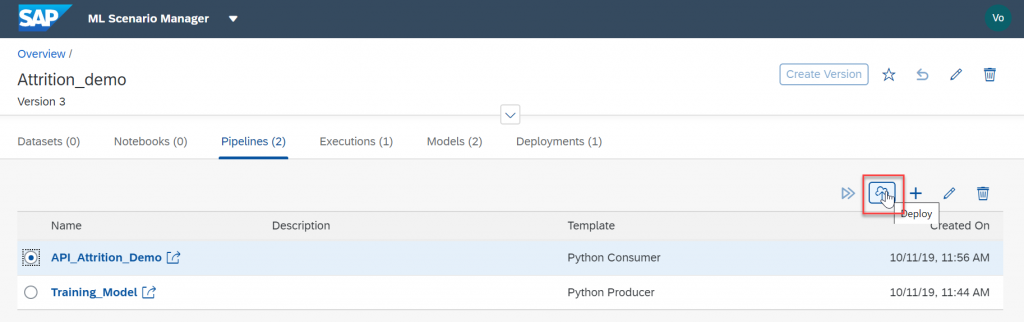
We now can deploy this pipeline, for this we will use the technical identifier of our previously training model.
Select your newly created pipeline and click the “Deploy” icon.
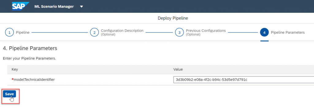
Go through all the step and when prompted for your modelTechnicalIdentifier enter the value of your model. Click "Save".
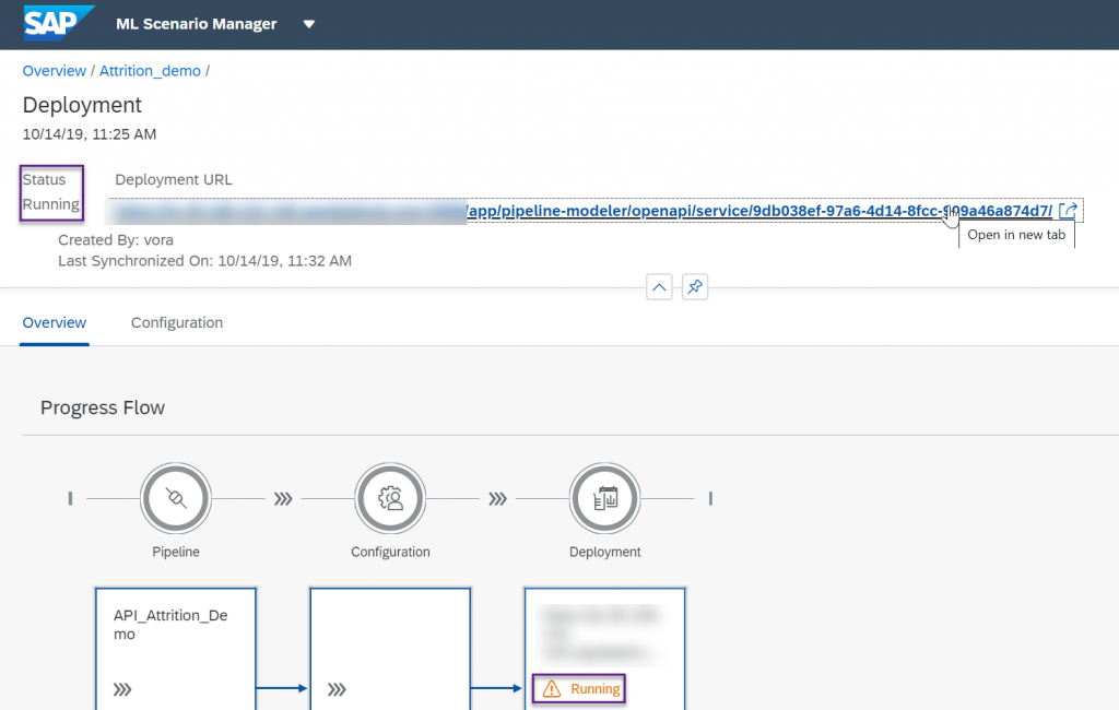
Deploy it, your status will be pending for a few minutes
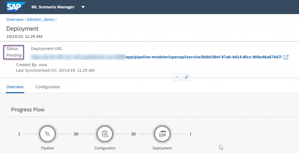
Once it is running, copy the URL of our deployed REST-API, don't try it as it is, it is missing some part.
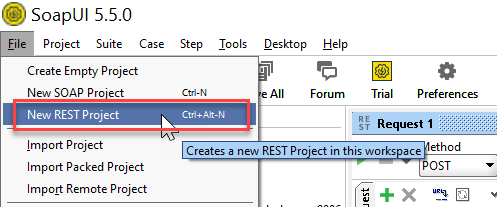
Contrary to Andreas who used Postman for his demo, my prefered tool is SoapUI. In a previous life, I found out some limits to Postman and have been using SoapUI ever since. It's more complex to use but has more features.
Open SoapUI and create a new REST project.
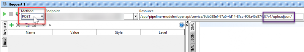
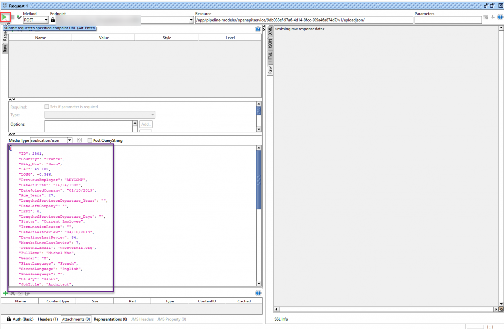
Add /v1/uploadjson/ to your deployed URL. Change the request type from “GET” to “POST”.
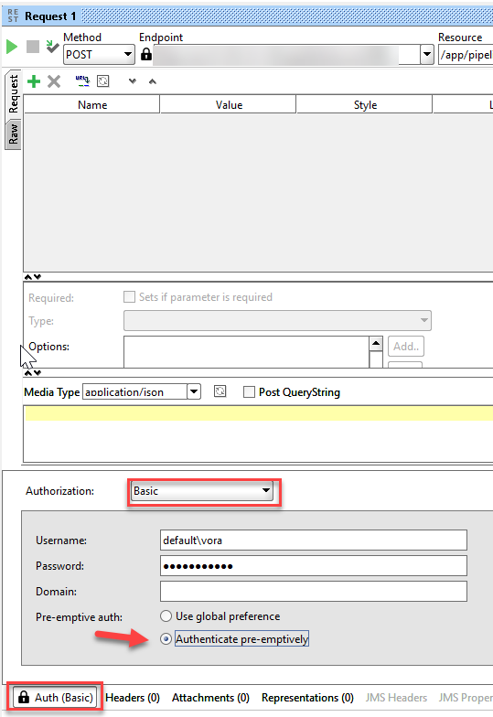
Go to the "Auth" tab below, select "Basic Authorization" and enter your user name and password for SAP Data Intelligence. The user name starts with your tenant’s name, followed by a backslash and your actual user name. For SoapUI we also need to select Authenticate pre-emptively.
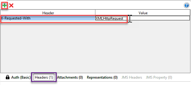
In the "Headers" tab and enter the key "X-Requested-With" with value “XMLHttpRequest”.
Then enter the input data in the REST-API:
{

    "ID": 2801,

    "Country": "France",

    "City_New": "Caen",

    "LAT": 49.182,

    "LONG": -0.366,

    "PreviousEmployer": "ANYCOMP",

    "DateofBirth": "16/04/1982",

    "DateJoinedCompany": "01/10/2019",

    "Age_Years": 27,

    "LengthofServiceonDeparture_Years": "",

    "DateLeftCompany": "",

    "LEFT": 0,

    "LengthofServiceonDeparture_Days": "",

    "Status": "Current Employee",

    "TerminationReason": "",

    "DateofLastreview": "04/10/2019",

    "DaysSinceLastReview": 84,

    "MonthsSinceLastReview": 7,

    "PersonalEmail": "whoever@if.org",

    "FullName": "Michel Who",

    "Gender": "M",

    "FirstLanguage": "French",

    "SecondLanguage": "English",

    "ThirdLanguage": "",

    "Salary": "34567",

    "JobTitle": "Architect",

    "VerbalCommunication": 4,

    "Teamwork": 4,

    "CommercialAwareness": 3,

    "AnalysingInvestigating": 4,

    "InitiativeSelfMotivation": 1,

    "Drive": 2,

    "WrittenCommunication": 2,

    "Flexibility": 4,

    "TimeManagement": 2,

    "PlanningOrganising": 3,

    "Phone": "000-000000",

    "EmployeeID": 12801,

    "Title": "M.",

    "UserID": "michelwho",

    "CompanyEmail": "mwho@anothercomp.org",

    "DaysSickYTD": 0,

    "FTEEquivalent": 1,

    "ContractedHoursperWeek": 37,

    "AverageWeeklyHoursWorkedYTD": 36.4,

    "ContractedHoursWorked": "98.00%",

    "AverageVariancefromContractedHoursYTD": "98%",

    "BirthCountry": "France",

    "InPensionScheme": "Y",

    "LastPayRise": 0,

    "LastPayRiseDate": "01/10/2019",

    "DaysWithoutRaise": 13,

    "PerformanceGrade2015": 0,

    "PerformanceGrade2014": 0,

    "JobType": "Skilled Labor",

    "QuarterofLastReview": 5,

    "YEARREVIEWPROS": "Managers that listen, plenty of O.T.",

    "YEARREVIEWCONS": "Company moves fast, so does the employees."

  }
Press the play button and you will get a result from our deployed model in SAP Data Intelligence.
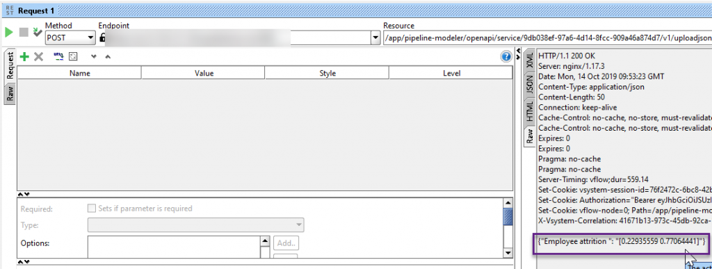
This specific employee has a 77.06% change of leaving us. Something needs to be done or we might loose him!
You can play around with the model by changing the values in our JSON request.
Summary
In this post, we used SAP Data Intelligence to create an attrition Data Science scenario. We used the embedded Jupyter Lab notebook to create our analysis and our Machine learning model. We then used this model in a provided template pipeline that we adapted to our business question. We then executed the model and validated that the model was accurate. With this pipeline, we will be able to recreate the model in case we identify a divergence between our predicted values and the real attrition in our company. We then created a second pipeline using another template to consume the previously created model and expose it as a REST API and then used a tool, such as SoapUI to run the model on employees.
I hope this tutorial was helpful, don't hesitate to comment if you need help or have questions.
- SAP Managed Tags:
- Machine Learning,
- SAP Data Intelligence
Labels:
4 Comments
You must be a registered user to add a comment. If you've already registered, sign in. Otherwise, register and sign in.
Labels in this area
-
ABAP CDS Views - CDC (Change Data Capture)
2 -
AI
1 -
Analyze Workload Data
1 -
BTP
1 -
Business and IT Integration
2 -
Business application stu
1 -
Business Technology Platform
1 -
Business Trends
1,661 -
Business Trends
87 -
CAP
1 -
cf
1 -
Cloud Foundry
1 -
Confluent
1 -
Customer COE Basics and Fundamentals
1 -
Customer COE Latest and Greatest
3 -
Customer Data Browser app
1 -
Data Analysis Tool
1 -
data migration
1 -
data transfer
1 -
Datasphere
2 -
Event Information
1,400 -
Event Information
64 -
Expert
1 -
Expert Insights
178 -
Expert Insights
273 -
General
1 -
Google cloud
1 -
Google Next'24
1 -
Kafka
1 -
Life at SAP
784 -
Life at SAP
11 -
Migrate your Data App
1 -
MTA
1 -
Network Performance Analysis
1 -
NodeJS
1 -
PDF
1 -
POC
1 -
Product Updates
4,577 -
Product Updates
324 -
Replication Flow
1 -
RisewithSAP
1 -
SAP BTP
1 -
SAP BTP Cloud Foundry
1 -
SAP Cloud ALM
1 -
SAP Cloud Application Programming Model
1 -
SAP Datasphere
2 -
SAP S4HANA Cloud
1 -
SAP S4HANA Migration Cockpit
1 -
Technology Updates
6,886 -
Technology Updates
402 -
Workload Fluctuations
1
Related Content
- Harnessing the Power of SAP HANA Cloud Vector Engine for Context-Aware LLM Architecture in Technology Blogs by SAP
- Adversarial Machine Learning: is your AI-based component robust? in Technology Blogs by SAP
- Possible Use Cases Of ECC & S/4HANA Connection With SAP Datasphere. in Technology Q&A
- Adversarial Machine Learning: is your AI-based component robust? in Technology Blogs by SAP
- SAP PI/PO migration? Why you should move to the Cloud with SAP Integration Suite! in Technology Blogs by SAP
Top kudoed authors
| User | Count |
|---|---|
| 12 | |
| 9 | |
| 7 | |
| 7 | |
| 7 | |
| 7 | |
| 6 | |
| 6 | |
| 6 | |
| 4 |