
- SAP Community
- Products and Technology
- Technology
- Technology Blogs by SAP
- Time Series Forecasting in SAP Analytics Cloud Sma...
Technology Blogs by SAP
Learn how to extend and personalize SAP applications. Follow the SAP technology blog for insights into SAP BTP, ABAP, SAP Analytics Cloud, SAP HANA, and more.
Turn on suggestions
Auto-suggest helps you quickly narrow down your search results by suggesting possible matches as you type.
Showing results for
Advisor
Options
- Subscribe to RSS Feed
- Mark as New
- Mark as Read
- Bookmark
- Subscribe
- Printer Friendly Page
- Report Inappropriate Content
10-07-2019
2:25 PM

Last update: This blog was updated last February 1st, 2023.
Overview
Time Series Forecasting is used to forecast the future evolution of a measure based on its past values. For example, how many products should be produced to cope with demand?
SAC (SAP Analytics Cloud) Smart Predict and Predictive Planning offer such forecasting capabilities. The high-level principle is that several predictive models are generated behind the scenes based on the three techniques shown in Fig. 1. All the predictive models that are generated enter a competition. At the end, only one predictive model is selected and presented to the end-user, the one with the best accuracy (in case of ex æquo, the most accurate and simplest model will be selected).

Fig 1: SAC Smart Predict time series forecasting process
The time series forecasting algorithm analyzes the time series and breaks it down into different components, easy to explain.
For the Additive technique, the time series is broken down into the following components:
Time series = Trend + Cycles + (Influencers) + Fluctuation + Residual
- Trend is the general orientation of the signal or its long-term evolution.
- Cycles correspond to periodic and/or seasonal events.
- Influencers indicates how the variable to forecast is influenced by other variables. This is an optional component which is present only if influencers are part of the predictive model.
- Fluctuation is what is left when the trend, the cycles (and optionally the influencers) have been extracted.
- Residual is what remains from the time series when all the above components have been subtracted from the original time series. This part of the data cannot be modelled and does not help determine predictive forecasts.
The resulting predictive model is a combination of the following components:
Predictive Model = Trend + Cycles + (Influencers) + Fluctuation
In 2020, the world entered a major crisis due to the COVID-19 pandemic. It affected all businesses. The pandemic peaks caused data disruption. You can read more here: Forecasting Time Series in COVID-19 Days.
If SAC Smart Predict detects various trends, it determines the change points and the corresponding trends, as shown in the figure below. Between the change points, the Piece-wise Trend Detection builds an additive predictive model to optimize at once the linear trends, cycles, fluctuation, and influencers.

Fig 2: Piecewise detection
Exponential Smoothing is a well-known technique that provides relevant and accurate predictive forecasts even on business time series that have been strongly disrupted. It gives more weight to the more recent observations compared to older observations. Exponential Smoothing provides better results when the amplitude of the cycles varies significantly.
SAC Smart Predict implements three kinds of exponential smoothing techniques. They are described in detail in this blog: Exponential Smoothing inside SAP Analytics Cloud time series forecasting scenarios.
- With Simple Exponential Smoothing, the predictive forecast at time t depends on actuals values at time t’<t multiplied by a smoothing factor.
- Ft= α [At-1 + (1 – α) At-2 + (1 – α)2 At-3 + … + (1 – α)t-2A1] + (1 – α)t A0
When the smoothing factor α is near 1, the weight of the oldest data is reduced, this gives a greater importance to recent data. Such technique is interesting in case of data disruption.
- Double Exponential Smoothing is an improvement of simple exponential smoothing when there is a trend in the data. The predictive forecast at time t depends on a level L used to measure how high the time series is and on the slope T of the trend.
- Ft= Lt + Tt
Where h is the number of forecasts requested in the future.
- Triple Exponential Smoothing is an improvement over simple and double exponential smoothing when there are cycles in the data. The predictive forecast at time t+k depends on a level L, on the slope T of the trend and on the cycles S.
- Ft+k= (Lt + kTt)St-M+k
Where k = 1 to the number of predictive forecasts requested in the future, and where M is a seasonality parameter that stands for the size of a cycle.
After the model selection step, the predictive model can generate predictive forecasts.
Predictive forecasts can be generated from predictive scenarios or stories and their generation can be scheduled using multi-actions.
You should have a good overview of SAC Smart Predict at this stage. If you need more details, please continue reading.
Which questions? Which data?
Time Series Forecasting is useful for estimating future values of a measure, let us see what kind of data the time series forecasting of SAC Smart Predict can handle Here are some typical questions related to time series forecasting:
- How will the revenue of my shop evolve over the next month?
- What are the expected sales by product per region for the next weeks?
- How will the stock of my products vary in my warehouse over the following weeks?
- How to predict the evolution of my cash flow during the next quarter?
Let us check if the type of data you have is usable for Time Series Forecasting. There are two distinct aspects:
- You must have recorded the values that your target variable had in the past and the corresponding dates. This couple (date, target value) is called the signal. This signal will be analyzed by the Time Series Forecasting process of SAC Smart Predict.
- Values of other variables for past and future dates can be included. These explanatory variables are called “Candidate Influencers.” They are used by SAC Smart Predict to refine the analysis of the signal. The blog Candidate Influencers in SAP Analytics Cloud Smart Predict explains how SAC Smart Predict uses these variables to improve the predictive forecasts.
Here is some advice to correctly prepare your data:
- Firstly, ask yourself how far into the future do I need to project? This is the horizon. It is the number of predictions you want to do in the future. This number depends directly on the size of your historical data. 5:1 is a good ratio to estimate the horizon and get predictions with relevant confidence intervals. This means that if you have 100 historical cases, you predict 20 values of your target variable in the future. Of course, the length of the horizon depends also on your use case, and you can choose less than 20 values. But if you need more, it will be better to collect more data history
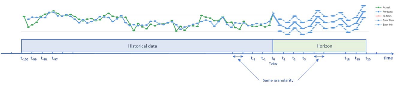
Fig 3: Signal and predictions on its evolution in the given horizon
- Secondly, you need to consider the scale of the predictions: every month, every week, every day, every hour. If your data history is captured every month, week, or day, then the predictions will be produced in the same unit of time. It seems evident that if you record values every month, it is not meaningful to request predictions for the next days! The opposite situation may arrive. For technical reasons if data is recorded every minute by sensors, but the minute is not relevant for your use case; then you need a higher unit of time like hour.
- Thirdly, if your business has been impacted by the pandemic and lockdown, you have observed a disruption in your data which could have taken several forms.
- A sharp drop of your business,
- After a lockdown, a slow recovery of activity,
- A behavior of customers at a smaller scale and quantity than before
These perturbations of business data lead to modifications of trends and cycles.
You will find a detailed analysis in the blog Forecasting Time Series in COVID-19 Days.
Candidate influencers are useful to increase the accuracy of the predictive model. Very often, these variables have a meaning only in your business domain and it will be necessary to manipulate your data to get them. Here are examples of such influencers:
- Specific selling periods for a product
- Time limit discount
- Monthly closing day / Quarterly closing day
- First day of month / Last day of the month
There are the constraints for candidate influencers to be used in the model:
- The future values must be known (at least for the expected horizon).
- Only candidate influencers with ordinal, and continuous types are used in the detection of cycles.
Use case : Optimize travel costs
We will follow a use case to illustrate this section, using a planning model with SAC Smart Predict to show you how the signal is processed to propose forecasts. This use case is about the travel costs of a company that has spun out of control, and negatively impacted the P&L (Profit & Loss) analysis and financial performance of the company. The company's objective is to analyze these costs and understand where they could be reduced but also to better forecast costs to avoid being over budget.
The data collected (see Fig. 4) in the past are:
- The posting period of travel costs collected every month from 2018 to 2022. It will be our date variable.
- The travel costs for each posting period. This is our target variable.
- The line of business (LOB) is also recorded because travel costs are not the same from one LOB to another.
- A series of influencers like Travel & Expense Budget, Software license sales targets per LOB per month or Number of existing headcounts and their associated budget. There are also candidate influencers related to time, like Number of working days in the month.

Fig 4: Planning model of the Travel costs use case
The graphical view of the signal for all LOB looks like Fig. 5. but each LOB has different travel consumption patterns. When travel cost is forecasted per LOB, then the analysis and the predictive forecasts become more accurate than the predictions obtained from a global predictive model and cascaded down to the different LOBs.
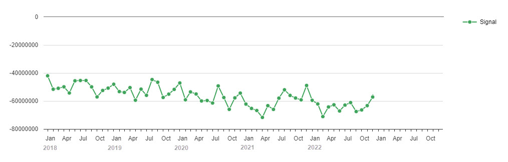
Fig 5: Signal for all the data
Time Series Modeling Process
The evolutions of the travel expenses are not the same for all the line of business (LOB). Having a predictive model specific for each LOB provides better accurate predictive forecasts than a unique model. To do that, there is an option (see Fig. 6) which allows us to select the variable for which we want to have a predictive model for each of its values.

Fig 6: Segmentation of the data on the values of the LOB
Concretely, what does this mean? In this time series, there are nine LOBS. SAC Smart Predict creates nine subsets of the data and generates nine predictive models. So, the predictions are specific to each LOB and are not influenced by the others.
As an example, here are the time series specific for the LOB “Cloud Services” (Fig. 7) and for LOB “Sales & Marketing” (Fig. 8).

Fig 7: Signal for Cloud Services

Fig 7: Signal for Cloud Services
A little bit of theory is necessary to understand how SAC Smart Predict generates the forecast for the travel costs use case.
For each of the LOB, SAC Smart Predict creates several predictive models. It uses three techniques:
- Additive technique
- Piece-wise Trend Detection
- Exponential Smoothing
These predictive models enter a competition and the most accurate and simplest one is selected at the end.
Now let us dig into more details of these techniques to understand how these predictive models are built.
Additive predictive model
The signal is broken out into four components which are:
- The Trend: This consists of finding out where your business is headed. In which direction it tends to go. Is it decreasing? Is it increasing?
- The Cycles patterns are Seasonality and Periodic Cycles. This means that they are reproduced regularly over time.
- The Influencers step consists in determining how additional variables influence the target when these variables exist in the data model.
- The Fluctuation creates a model of the dependencies of the values at time “t” with previous values.
- Finally, the Residuals are what remains of the signal when Trends, Cycles and Fluctuations have been removed. Residuals are considered as “white noise”; this means that they are purely random effects.
At the end, SAC Smart Predict combines the models of each combination to find the best model.
This process is summarized in Fig. 9.

Fig 9: Smart Predict process to handle a time series forecasting signal
Let us see in more detail each of these four steps of the time series process in SAC Smart Predict.
Trend detection
The first step is to determine the best trend of the signal. The trend is the general orientation of the signal or its long-term evolution. To obtain the trend shown in Fig. 10, SAC Smart Predict puts several trends in competition. Note that no choice is made at this step before the estimation of the other components of the signal. The LEAN project introduced in the blog is the result of our research to improve both the performance of the predictive models and their explainability.

Fig 10: Linear trend of LOB Operations
Here are the four main methods to determine the trends.
- Lag 1 (L1) - The assumption is that forecast at time t will depend on the past values of the signal. The signal moved one step forward. This is the basic forecast where the predicted observation equals the latest signal observation.
Trendt = Yt-1
For the other methods, the assumption is that the forecast at time t is independent of any past values of the signal. The SAC Smart Predict regression algorithm is used for that but, it is based on three different inputs:
- Date: A0 and A1 are estimated with Yt as target variable and Time as input variable.
Trendt = A0 + A1Time - Date, Candidate influencer variables: A0, A1, B1, B2, … are estimated with Yt as target variable and Time, X1, X2, … as extra-predictable variables
Trendt = A0+ A1Time + B1 X1 + B2 X2 + … - Candidate influencer variables: X1, X2, … as candidate influencer variables
Trendt = B1 X1 + B2 X2 + …
Detection of Cycles
The second step consists in determining the existing cycles in the signal. To obtain the cycles shown in Fig. 11, SAC Smart Predict iterates to detect all cycles.

Fig 11: Cycle of LOB HR (Human Resource)
There are two main types of cycles:
- Periodicity which describes natural events which reproduce themselves at a fixed interval of time called a period.
- Seasonality which describes calendar events: 13 types of seasonalities are examined.
Cycles of both types are computed through an encoding of the signal. For periodicity, the encoding is based on a period length. With a period equals to 5, the encoding will be 0, 1, 2, 3 and 4 and the value will be the average signal observed on every 5th step. SAC Smart Predict can automatically test up to 450 different periods. The encoding for seasonality is based on calendar events.
Cycles are also evaluated on candidate influencers. For this, the encoding depends on the variable type.
- For nominal variables: no encoding done, thus no cycle detected.
- For ordinal and continuous variables: encoding done on the natural order
The time series is split into two subsets. The estimation subset is used to detect cycles and the validation subset is used to check accuracy of cycles. It is important to reduce the scope of cyclic search to minimize the computation time and particularly for periodicities. Thus, the maximum length of a period is by default equal to the minimum between 1/12 of the estimation subset size and 450.
You need to have enough historical data to detect cycles and particularly cycles or seasonality’s over extended periods.
At this step all the encodings done are cycle candidates and it is time to put them in competition to select one. To do this, SAC Smart Predict runs this iterative process:
- For each of the detected trends, the signal Yt is detrended to produced Yt – Trendt
- For each candidate cycle Cyclet
- Measures the link between the signal Yt – Trendt and Cyclet
- If this improves the forecast (comparison of actual and forecasted value in the validation subset) then analysis is repeated on Trendt + Cyclet
- Else reject Cyclet
The selection process stops when there is no significant cycle to add to the predictive model.
Influencers detection
Trend and cycles detections are based on the evolution of the target's values over time. If you have measured other variables, SAC Smart Predict can use them to measure how they could impact the target. This refines the predictive model and gives you information about your data that you did not suspect. At the bottom right of Fig. 12 below you list the variable of the data model that are candidate influencers. Once the predictive model is built, the influencers are displayed in the Explanation panel. Here we see that travel cost for LOB Accounting & Finance is influenced at 32.92% by variable GPO Rebates ACT.

Fig 12: Impact of influencers on LOB Accounting & Finance
Note that to be a candidate influencer, it is mandatory to know its future values (at least for the expected number of predictions). To know more about influencers, you can read this blog.
Fluctuation detection
The third step consists in determining fluctuation of the signal. The fluctuation is what is left when the trend and the cycles have been extracted. To obtain the fluctuation shown in Fig. 13, SAC Smart Predict creates an auto-regressive model that uses a window of past data to model the remaining signal.

Fig 13: Fluctuation of LOB Operations
At this stage, the initial signal has been broken out and removed its trend, cycles and potentially influencers: Signal – Trend – Cycles - Influencers. An auto-regressive model is then computed on what is left from the signal:
Xt = a0 Xt-1 + a2 Xt-2
Where p is called the order of the auto-regressive model. This order is limited to 2. This allows to better detect cycles than fluctuations which are more difficult to interpret. The additional effect is to increase the explainability of the predictive model because we see more often the impact of cycles.
At the end, when trend, cycles and fluctuation are removed from the original signal, the only points which persist are the residual which are considered as noise. Fig. 14 shows such residuals.
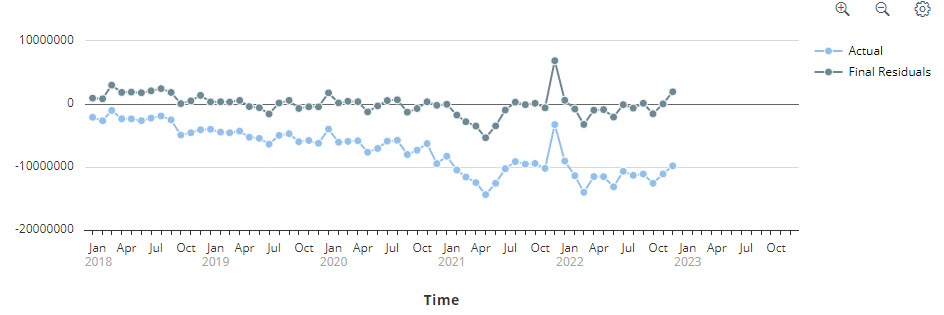
Fig 14: Residuals of LOB Cloud Services
Piece-wise Trend Detection
This technique was introduced in SAC Smart Predict after the first lockdown due to the Covid-19 pandemic. The clear objective was to reduce the effect of the disruption observed in the data (see Fig. 14) and get again accurate predictive forecasts.
The first step of the Piece-wise Trend detection is to discover the points where a disruption starts and ends. These points are called the changed points. Their detection is based on a complex optimization of a cost function which considers at the same time, the quadratic error, and the linear alignment of the successive points.
The second step consists in splitting the signal from a change point to the next one and using the additive method of each segment to determine trends. Cycles, fluctuation, and influencers are determined on the complete signal. The final predictive model is the union of each of these components. Fig. 15 below is an example for such predictive model.

Fig 15: Piece-wise trend predictive model
Exponential Smoothing
This technique can be robust in the presence of disruption and gives more weight to recent data. Fig. 16 shows the breakdown of a time series breakdown with this technique.

Fig 16: Exponential smoothing technique used for this predictive model
To get a complete explanation of Exponential Smoothing, refer to this blog.
Predictive Model Selection
Now that SAC Smart Predict has determined a set of candidate predictive models, it is time to select the best one. During the training time, the initial signal Yt was broken out specific components:
- In trends, cycles, fluctuations, residuals, and influencers for additive and piece-wise trend
- In level, slope, and cycles for exponential smoothing
For the additive modeling technique, the remaining signal after removing the trends, the cycles, the influencers, and the fluctuations, represents the residues. After trying several combinations of models, the final selected model is the one whose residues are statistically uncorrelated (the closest possible to white noise).
Now that the components of the signal have been determined, SAC Smart Predict compares the models of each combination to find the best model, using a quality indicator and a validation process.
The historical data is split into two parts: 75% are reserved to study the signal and generate the models as seen previously. The 25% which remains constitutes the validation subset and is used to measure the quality of the candidate models so that the best can be selected.
The validation process compares the actual values of the measure with the values predicted by each model. A measure called Mean Absolute Error (MAE) is computed with this formula. It is the average of the absolute difference between the predictions done by a model and the actual values.

Now in the input parameter of a forecast, you specify several forecast periods (this corresponds to the horizon noted H). This is the distance in the future where SAC Smart Predict predicts values for you. For each model, SAC Smart Predict computes several individual MAE values corresponding to the requested forecasts periods and computes their average. The computed result is the Average Expected MAE

To select the best model, SAC Smart Predict is doing a combination of these two indicators:
- The performance measured by the Average Expected MAE: The predictive model with the best Average Expected MAE is selected.
- The complexity of the model: In the event of a tie, with a 5% tolerance, the simplest predictive model is the winner.
Quality of the Predictive Model
Note that the MAE and Average Expected MAE are internal measures and are not surfaced in SAC Smart Predict to date. The quality indicator surfaced in SAC Smart Predict is based on another metric called the Average Expected MAPE (Mean Absolute Percentage Error) because the MAPE is a kind of standard in the market.
To get it, the individual MAPE is computed by this formula.

It measures the accuracy of the model’s forecasts and indicates how much the forecast differs from the real signal value.
To consider the horizon, SAC Smart Predict computes for each model, several individual MAPE corresponding to the requested horizon and takes their average. It is the Average Expected MAPE

How to interpret the Average Expected MAPE? It is expressed in percentage. A zero percent value indicates a perfect model. A value of 10% means that the error done when using the predictive forecast is 10%. Values above 100% are the subject of discussion. You need to compare the predictive model and its forecasted values with your business knowledge to decide about its accuracy. You can get detailed explanations on MAPE in this blog.
We have introduced a quality indicator: Median Expected MAPE. It is useful on a predictive model with several entities to avoid being influenced by extreme values. The median is complementary to the average and provides a better indication of the overall model performance. In Fig. 18 below, we see Expected MAPE of the LOB Board of Directors, Accounting & Finance and Purchasing are not particularly good while the performance of the other predictive models of the other LOB are much better. If you look only at the Average Expected MAPE, you could conclude that the model will deliver a mediocre performance. While looking at the Median Expected MAPE, you see that the performance is much better.
Using the forecasting model
Now that we know how SAC Smart Predict builds a forecasting model, we can run it on the travel costs data with these input parameters (Fig. 17).
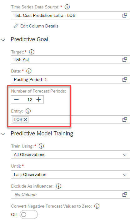
Fig 17: Input parameters
You will notice that:
- The forecasting is segmented on the 9 values of the LOB so that 9 predictive models will be generated.
- The horizon for all the forecasts is 12 months. It is month because the granularity of the training subset is the month.
Once the training process is complete, an overview allows you to see the quality of the models per board area as shown in Fig. 18.

Fig 18: Global Quality indicators and per LOB.
Immediately you see the quality of the predictive models selected for all LOB. Here the predictive model that will provide the most accurate predictive forecasts is the one for the LOB Sales & Marketing. You get the details for this LOB when you click on it as shown in Fig. 19.
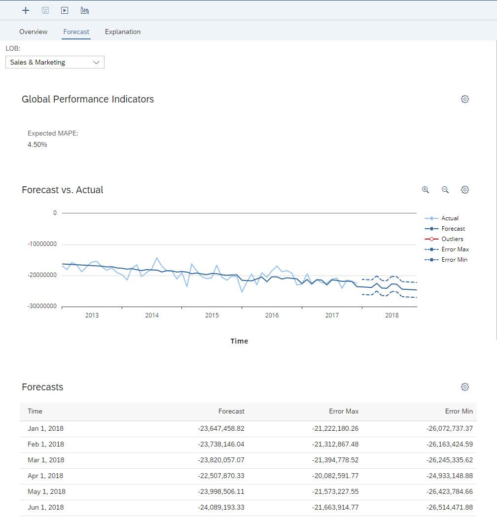
Fig 19: Forecast for segment Sales & Marketing
The legend of the chart indicates in light blue the actual values for this LOB. In blue, it is the 12 forecasted values with their error min and max.
A table of the forecasted values is at the bottom.
When you click on the Save Forecast button, the forecasted values are output in a planning model version as shown in Fig. 20.
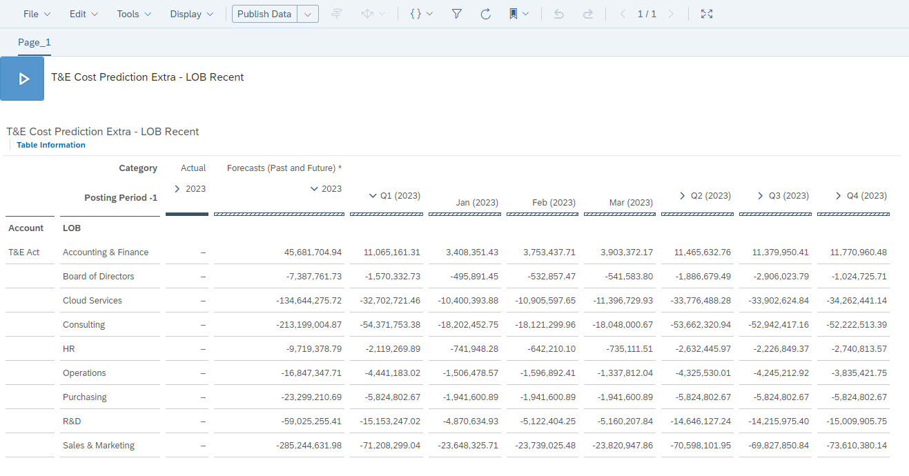
Fig 20: Forecasted values applied saved into a planning model
Conclusion
I hope you now have a better understanding of the SAC Smart Predict process to provide relevant forecasts.
Resources to learn more about SAC Smart Predict.
- Hands-On Tutorial SAP Smart Predict, Product Forecast
- Understand accuracy measure of time series forecasting models
- SAC Predictive Planning blogs
Finally, if you enjoyed this post, I would be grateful if you would help it spread, comment and like. Thank you!
- SAP Managed Tags:
- SAP Analytics Cloud,
- SAP Analytics Cloud, augmented analytics
Labels:
40 Comments
You must be a registered user to add a comment. If you've already registered, sign in. Otherwise, register and sign in.
Labels in this area
-
ABAP CDS Views - CDC (Change Data Capture)
2 -
AI
1 -
Analyze Workload Data
1 -
BTP
1 -
Business and IT Integration
2 -
Business application stu
1 -
Business Technology Platform
1 -
Business Trends
1,661 -
Business Trends
86 -
CAP
1 -
cf
1 -
Cloud Foundry
1 -
Confluent
1 -
Customer COE Basics and Fundamentals
1 -
Customer COE Latest and Greatest
3 -
Customer Data Browser app
1 -
Data Analysis Tool
1 -
data migration
1 -
data transfer
1 -
Datasphere
2 -
Event Information
1,400 -
Event Information
64 -
Expert
1 -
Expert Insights
178 -
Expert Insights
270 -
General
1 -
Google cloud
1 -
Google Next'24
1 -
Kafka
1 -
Life at SAP
784 -
Life at SAP
11 -
Migrate your Data App
1 -
MTA
1 -
Network Performance Analysis
1 -
NodeJS
1 -
PDF
1 -
POC
1 -
Product Updates
4,578 -
Product Updates
323 -
Replication Flow
1 -
RisewithSAP
1 -
SAP BTP
1 -
SAP BTP Cloud Foundry
1 -
SAP Cloud ALM
1 -
SAP Cloud Application Programming Model
1 -
SAP Datasphere
2 -
SAP S4HANA Cloud
1 -
SAP S4HANA Migration Cockpit
1 -
Technology Updates
6,886 -
Technology Updates
395 -
Workload Fluctuations
1
Related Content
- ML- Linear Regression definition , implementation scenarios in HANA in Technology Blogs by Members
- Planning Professional vs Planning standard Capabilities in Technology Q&A
- Forecast Local Explanation with Automated Predictive (APL) in Technology Blogs by SAP
- What’s New in SAP Analytics Cloud Release 2024.07 in Technology Blogs by SAP
- Unleashing AI and Machine Learning in Sales: Advanced Price-Volume Forecasting with SAP Analytics Cl in Technology Blogs by SAP
Top kudoed authors
| User | Count |
|---|---|
| 11 | |
| 10 | |
| 10 | |
| 9 | |
| 8 | |
| 7 | |
| 7 | |
| 7 | |
| 7 | |
| 6 |