
- SAP Community
- Products and Technology
- Technology
- Technology Blogs by SAP
- Train and Deploy a Tensorflow Pipeline in SAP Data...
Technology Blogs by SAP
Learn how to extend and personalize SAP applications. Follow the SAP technology blog for insights into SAP BTP, ABAP, SAP Analytics Cloud, SAP HANA, and more.
Turn on suggestions
Auto-suggest helps you quickly narrow down your search results by suggesting possible matches as you type.
Showing results for
Advisor
Options
- Subscribe to RSS Feed
- Mark as New
- Mark as Read
- Bookmark
- Subscribe
- Printer Friendly Page
- Report Inappropriate Content
09-30-2019
1:08 PM
SAP Data Intelligence allows for scaling the AI capabilities in the enterprise collaboratively. It provides an end-to-end tool for managing machine learning models effectively with built-in tools for data governance and lifecycle management.
The aim of this blog post is to describe the necessary steps for provisioning and maintaining a machine learning service. This includes the typical phases of a data-science project:
A data scientists typically tackles a machine learning task by starting with experiments in Jupyter notebooks. He needs to store the data e.g. in DataLake. When finished with experiments the service needs to be productized.
You will learn how to set up a training and inference pipeline. Finally, in order to test the deployed ML service you will use simple ways to simulate a REST client.
The ML Scenario Manager supports also the lifecycle management of an ML service. Models can be trained on new data and be redeployed. The versioning makes sure that every step is reproducible.
This blog post extends the blog post SAP Data Intelligence: Create your first ML Scenario by using Tensorflow for training and serving a machine learning model.
Note: GPU based training is not covered here. The MLF Training operator leverages the power of GPUs, whereas the plain Python operator cannot do this.
The Iris dataset contains 150 records with 4 petal attributes and the corresponding Iris species name. The attributes which are used for training are Petal Length, Petal Width, Sepal Length, Sepal Width.
The "ML Scenario" represents the data-science project and includes everything for productizing an ML service and maintaining its lifecycle.
The training data in the Data Lake storage can be versioned to make sure that the models created by the training pipeline are reproducible.
Therefore we will register the dataset as an artifact for this ML Scenario.

A Jupyter notebook provides a great way to prepare the data and test the python / tensorflow code for training a neural network.
As the network achieves a 96% accuracy on the test data, we are ready to productize the code into a training pipeline.

The training pipeline used here creates the model artifact. This is a necessary step in terms of lifecycle management as it allows for reproducing the artifact.
The plain Python operator is based on a docker image that does not include libraries like tensorflow. Therefore, we need to build a custom docker, where our code can be executed.
Follow the steps in the blog post SAP Data Hub – Develop a custom Pipeline Operator with own Dockerfile (Part 3) (only section "1. Create a Dockerfile". We will not create a custom operator.)
The dockerfile looks like this and the tags that need to be added are listed in the Tags.json. (Note: add one tag in the config panel and save. Then you can edit the Tags file right below the Docker file in the "repository panel" on the left. Copy and paste the whole Tags.json.)

Hint: the last tag which is called "iris" is only used to make our tag list unique. We will later use this tag to reference our custom docker.
The training pipeline will read the data from DataLake using the "Read File" operator and feed it into the Python3 operator containing the training code.
If one prefers to read the data in chunks, alternatively one could read the data in the Python3 operator using sapdi sdk.
The resulting model is registered as an artifact for this ML Scenario by the "Artifact Producer".
We need to perform a couple of modifications before we can run the tensorflow code from the Experiment, i.e. the Jupyter notebook.
The data is passed as messages between the operators. Therefore we need to modify the Jupyter notebook code. Rather than reading the training data from a file, the message passed to the "on_input" method is processed by a stream reader.
This triggers the execution of the pipeline.
The 2 input parameters are displayed because the Read File operator contains a variable for the file path (for the registered dataset in DataLake)

and the Artifact Producer a variable for the Artifact Name, i.e. the trained model.

When the training pipeline is completed you will see the result in Scenario Manager, where the metrics (accuracy: 96%) and the model are displayed.
Click the arrows in the final step "Model and Datasets" to jump to the registered model artifact by the name of "iris". We will use this model artifact for deploying the Iris classification service.
Hint: use the zoom button to the right if the details are not displayed.

In order to provide a REST endpoint for the Iris classifier based on the model trained in the previous step, we will deploy a pipeline, that accepts input data and returns the classified Iris flower category.
The inference pipeline includes a REST server with the option to define the paths using swagger. It accepts the input data as json and after having loaded the iris model it will perform the prediction and return the result.

The Iris classification service is deployed and ready for serving!

As the training data was scaled between 0 and 1, we need to do the same with the data we send to the service for classification (see Jupyter notebook below).
For testing the deployed service one could build a REST client or use the sample Postman collection (import into postman and adjust request url and username / password).
It is also possible to test the endpoint in Jupyter Lab:
For path /v1/predict the the probabilities for each class is displayed, whereas /v1/predict_classes shows the iris category 0, 1, or 2 per test input.

Now you have completed implementing the scenario. In the Scenario Manager - Overview you can see all scenarios. Select the "Iris" scenario to display the versions.
Click on a version to access e.g. a pipeline state at any given step of the implementation of this scenario.
This blog post covered the aspects and details of setting up and running a Tensorflow based Machine Learning service. With SAP Data Intelligence such a service can easily be used both by users inside an enterprise and by its customers.
Machine Learning models can degrade over time. Therefor, it is vital to support the lifecycle management by retrieving and adapting the versioned pipelines of a given ML service easily. In order to update the service, the data-scientist does not depend on the support of IT, she can rather (re-)deploy the service in a one-click manner.
The aim of this blog post is to describe the necessary steps for provisioning and maintaining a machine learning service. This includes the typical phases of a data-science project:
- Data Preparation
- Experiments
- Model Development
- Deployment
- Lifecycle Management
A data scientists typically tackles a machine learning task by starting with experiments in Jupyter notebooks. He needs to store the data e.g. in DataLake. When finished with experiments the service needs to be productized.
You will learn how to set up a training and inference pipeline. Finally, in order to test the deployed ML service you will use simple ways to simulate a REST client.
The ML Scenario Manager supports also the lifecycle management of an ML service. Models can be trained on new data and be redeployed. The versioning makes sure that every step is reproducible.
This blog post extends the blog post SAP Data Intelligence: Create your first ML Scenario by using Tensorflow for training and serving a machine learning model.
Note: GPU based training is not covered here. The MLF Training operator leverages the power of GPUs, whereas the plain Python operator cannot do this.
Contents
- Upload Data
- Create Machine Learning Scenario
- Experiments
- Build Training Pipeline
- Deploy service as REST Api
- Simple Client for Testing the Service
- Conclusion
1. Upload Data
The Iris dataset contains 150 records with 4 petal attributes and the corresponding Iris species name. The attributes which are used for training are Petal Length, Petal Width, Sepal Length, Sepal Width.
- Copy the raw data into a text file and save as "iris.csv".
- In the SAP Data Intelligence Launchpad select Metadata Explorer and click on "Browse Connections".

- Select the "Connection to DI Data Lake; Type: SDL"
Prerequisite: In the Connection Management app the SDL (SAP Data Lake) connection type is enabled. - Select the "worm" (write once, read multiple) folder. This is used for immutable artifacts and data.
Note: "worm" will be deprecated in 2020. Use "shared" instead. - Create the folder "iris" for storing data related to this project.
- Click the "iris" folder to upload the file "iris.csv" created earlier.
2. Create Machine Learning Scenario
The "ML Scenario" represents the data-science project and includes everything for productizing an ML service and maintaining its lifecycle.
- Start ML Scenario Manager in the DI launchpad.
- Click the "+" sign to create an ML Scenario and provide a name e.g. "Iris - flower classification"
Register the dataset
The training data in the Data Lake storage can be versioned to make sure that the models created by the training pipeline are reproducible.
Therefore we will register the dataset as an artifact for this ML Scenario.
- In the "Datasets" section click the "+" sign to register the iris dataset:
enter a name and "dh-dl://worm/iris/iris.csv" as the url.
Note: "worm" will be deprecated in 2020. Replace with "shared". - Click on "Create Version" in the top right. This creates a snapshot of the current ML scenario.
3. Experiments
A Jupyter notebook provides a great way to prepare the data and test the python / tensorflow code for training a neural network.
- In the "Notebooks" section click the "+" sign and provide a name.
- In Jupyter Lab click the notebook and select "Python3" as kernel.
- Copy the code from keras.ipynb.
- Run "All Cells" from the Jupyter menu
As the network achieves a 96% accuracy on the test data, we are ready to productize the code into a training pipeline.
- Close the Jupyter Lab tab.
- In the Scenario Manager click "Create Version"
4. Build Training Pipeline
The training pipeline used here creates the model artifact. This is a necessary step in terms of lifecycle management as it allows for reproducing the artifact.
Build a Custom Docker
The plain Python operator is based on a docker image that does not include libraries like tensorflow. Therefore, we need to build a custom docker, where our code can be executed.
Follow the steps in the blog post SAP Data Hub – Develop a custom Pipeline Operator with own Dockerfile (Part 3) (only section "1. Create a Dockerfile". We will not create a custom operator.)
The dockerfile looks like this and the tags that need to be added are listed in the Tags.json. (Note: add one tag in the config panel and save. Then you can edit the Tags file right below the Docker file in the "repository panel" on the left. Copy and paste the whole Tags.json.)
Hint: the last tag which is called "iris" is only used to make our tag list unique. We will later use this tag to reference our custom docker.
Create the Training Pipeline
- In Scenario Manager go to the Pipelines section and click on the "+" sign
- Enter "train" as name and an optional description, e.g. "training pipeline"
- Select the "Python Producer" Template.
- Click Create which will open the pipeline modeler.
- Click the "Read File" operator and open the "Configuration" (graph toolbar button on right).
- In the "Service" dropdown, choose "SDL" (Semantic Data Lake)
Note: the "Path" entry "${inputFilePath}" acts as an input variable when the pipeline is executed.
The training pipeline will read the data from DataLake using the "Read File" operator and feed it into the Python3 operator containing the training code.
If one prefers to read the data in chunks, alternatively one could read the data in the Python3 operator using sapdi sdk.
The resulting model is registered as an artifact for this ML Scenario by the "Artifact Producer".
We need to perform a couple of modifications before we can run the tensorflow code from the Experiment, i.e. the Jupyter notebook.
- Right-click the Python3 operator which connects to "Submit Metrics" and "Artifact Producer" and select "Group".
This creates a separate docker for the operator. - Click the "Group" and select the small icon called "Open Configuration"
- In the Configuration panel on the right add the tag "iris" by selecting it from the left dropdown list.
Note: this is the extra tag we added while building the custom docker. Alternatively we could list all tags used for the custom docker. As long as no other "iris" tag is applied to another datahub docker we are safe.
The data is passed as messages between the operators. Therefore we need to modify the Jupyter notebook code. Rather than reading the training data from a file, the message passed to the "on_input" method is processed by a stream reader.
- Click the Python3 operator that uses our custom docker, i.e. the Group with the "iris" tag.
- Select the "Script" icon to open the code in a separate tab.
- Remove the code and replace by the train-operator.py code.
- Close the python operator code tab.
- Click the Save button at the toolbar on top of the pipeline graph.
- Close the browser tab containing the pipeline modeler.
Note: this will trigger an update for Scenario Manager to enable the "Create Version" button. - In Scenario Manager click "Create Version".
Execute Training Pipeline
- In Scenario Manager select the "train" pipeline (option button) and click on the "Execute" button in the Pipelines section.
- Click through steps 2 and 3.
- In Step 4 enter:
"iris" (without quotes) for the "newArtifactName and - "/worm/iris/iris.csv" (again without quotes) for the "inputFilePath"
Note: "worm" will be deprecated in 2020. Replace with "shared". - Click Save (only once!)
This triggers the execution of the pipeline.
The 2 input parameters are displayed because the Read File operator contains a variable for the file path (for the registered dataset in DataLake)
and the Artifact Producer a variable for the Artifact Name, i.e. the trained model.
When the training pipeline is completed you will see the result in Scenario Manager, where the metrics (accuracy: 96%) and the model are displayed.
Click the arrows in the final step "Model and Datasets" to jump to the registered model artifact by the name of "iris". We will use this model artifact for deploying the Iris classification service.
Hint: use the zoom button to the right if the details are not displayed.
5. Deploy service as REST Api
In order to provide a REST endpoint for the Iris classifier based on the model trained in the previous step, we will deploy a pipeline, that accepts input data and returns the classified Iris flower category.
Build the Inference Pipeline
The inference pipeline includes a REST server with the option to define the paths using swagger. It accepts the input data as json and after having loaded the iris model it will perform the prediction and return the result.
- In Scenario Manager go to the Pipelines section and click on the "+" sign
- Enter "inference" as name and an optional description, e.g. "iris classification".
- Select the "Python Consumer" Template.
- Click "Create" which opens the pipeline modeler.
- Select the "OpenApi Servlow" operator and click the icon "Open Configuration"
- Replace the content of the "swagger Spec" with iris-swagger.json.
It includes 2 paths: "/v1/predict" and "v1/predict_classes" which we will be used in the REST client. - Open the configuration for the "Submit Artifact Name" operator.
- Add the registered model name to the variable in the "Content" property:
${ARTIFACT:MODEL:iris} - Right-click the "Python36 Inference" operator and select "Group".
- Open the Group's configuration.
- Add "iris" (without quotes) in the Tags property (same as we did for the Training pipeline).
- Click the "Python36 Inference" operator and select the "Script" icon.
- In the code tab remove the code and insert the inference-operator.py code.
Note: make sure to create a new Message instance when sending back the result. - Close the code tab in pipeline modeler (not the browser tab!).
- Click the Save button at the toolbar on top of the pipeline graph.
- Close the browser tab containing the pipeline modeler.
- In Scenario Manager click on "Create Version".
Deploy the Inference Pipeline
- In Scenario Manager select the "inference" pipeline (option button) and click on the "Deploy" button (next to "Execute") in the Pipelines section.
- Click through steps 2 - 3.
- In Step 4 select (the most recent) trained "iris" model form the dropdown list.
- Click Save (only once!)
The Iris classification service is deployed and ready for serving!
- Copy the Deployment URL
6. Simple Client for Testing the Service
As the training data was scaled between 0 and 1, we need to do the same with the data we send to the service for classification (see Jupyter notebook below).
For testing the deployed service one could build a REST client or use the sample Postman collection (import into postman and adjust request url and username / password).
It is also possible to test the endpoint in Jupyter Lab:
- In Scenario Manager add a new notebook e.g. "inference-client.ipynb"
- Add the code from here.
- Fill in user, password and Deployment URL (see previous section)
- Run all cells
Every execution selects randomly test data. - Change the the path to /v1/predict_classes
- Run all cells
For path /v1/predict the the probabilities for each class is displayed, whereas /v1/predict_classes shows the iris category 0, 1, or 2 per test input.
- Close the Jupyter Lab browser tab.
- In Scenario finally click "Create Version".
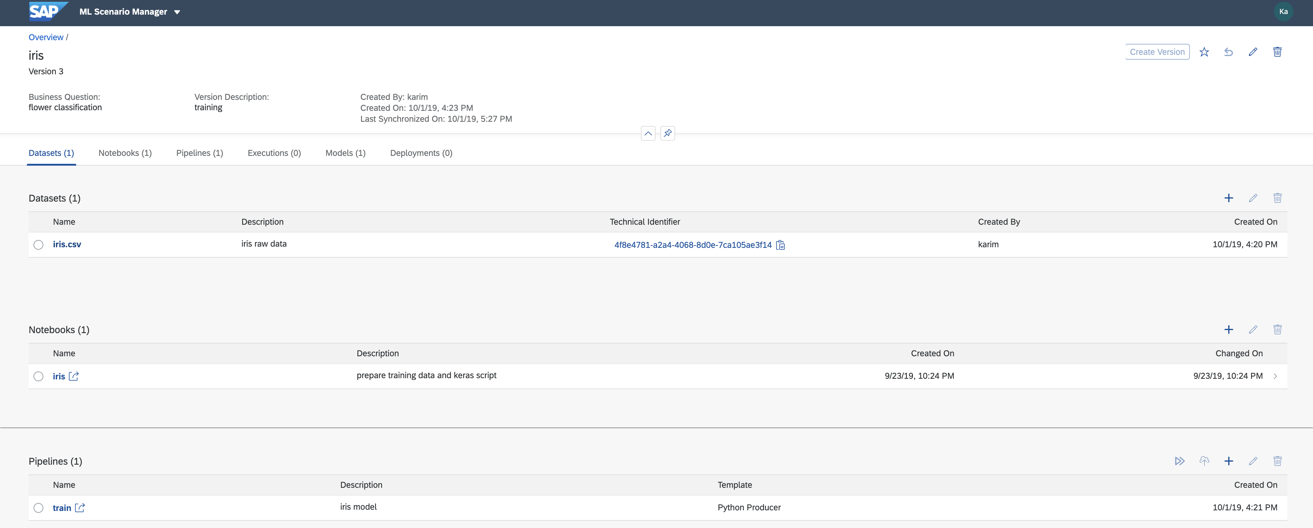
Now you have completed implementing the scenario. In the Scenario Manager - Overview you can see all scenarios. Select the "Iris" scenario to display the versions.
Click on a version to access e.g. a pipeline state at any given step of the implementation of this scenario.
7. Conclusion
This blog post covered the aspects and details of setting up and running a Tensorflow based Machine Learning service. With SAP Data Intelligence such a service can easily be used both by users inside an enterprise and by its customers.
Machine Learning models can degrade over time. Therefor, it is vital to support the lifecycle management by retrieving and adapting the versioned pipelines of a given ML service easily. In order to update the service, the data-scientist does not depend on the support of IT, she can rather (re-)deploy the service in a one-click manner.
- SAP Managed Tags:
- Machine Learning,
- SAP Data Intelligence
Labels:
15 Comments
You must be a registered user to add a comment. If you've already registered, sign in. Otherwise, register and sign in.
Labels in this area
-
ABAP CDS Views - CDC (Change Data Capture)
2 -
AI
1 -
Analyze Workload Data
1 -
BTP
1 -
Business and IT Integration
2 -
Business application stu
1 -
Business Technology Platform
1 -
Business Trends
1,661 -
Business Trends
87 -
CAP
1 -
cf
1 -
Cloud Foundry
1 -
Confluent
1 -
Customer COE Basics and Fundamentals
1 -
Customer COE Latest and Greatest
3 -
Customer Data Browser app
1 -
Data Analysis Tool
1 -
data migration
1 -
data transfer
1 -
Datasphere
2 -
Event Information
1,400 -
Event Information
64 -
Expert
1 -
Expert Insights
178 -
Expert Insights
274 -
General
1 -
Google cloud
1 -
Google Next'24
1 -
Kafka
1 -
Life at SAP
784 -
Life at SAP
11 -
Migrate your Data App
1 -
MTA
1 -
Network Performance Analysis
1 -
NodeJS
1 -
PDF
1 -
POC
1 -
Product Updates
4,577 -
Product Updates
329 -
Replication Flow
1 -
RisewithSAP
1 -
SAP BTP
1 -
SAP BTP Cloud Foundry
1 -
SAP Cloud ALM
1 -
SAP Cloud Application Programming Model
1 -
SAP Datasphere
2 -
SAP S4HANA Cloud
1 -
SAP S4HANA Migration Cockpit
1 -
Technology Updates
6,886 -
Technology Updates
407 -
Workload Fluctuations
1
Related Content
- ML Scenario Implementation (Logistics Regression Model) using SAP Data Intelligence in Technology Blogs by Members
- SAP Inside Track Bangalore 2024: FEDML Reference Architecture for Hyperscalers and SAP Datasphere in Technology Blogs by SAP
- Replication Flow Blog Series Part 5 – Integration of SAP Datasphere and Databricks in Technology Blogs by SAP
- What's the successor off Data Intelligence for Data Integration ? in Technology Q&A
- Unleashing the Power of SAP AI Launchpad & SAP AI Core: Create Your First AI Project in Technology Blogs by Members
Top kudoed authors
| User | Count |
|---|---|
| 13 | |
| 10 | |
| 10 | |
| 7 | |
| 7 | |
| 6 | |
| 5 | |
| 5 | |
| 5 | |
| 4 |