
- SAP Community
- Products and Technology
- Technology
- Technology Blogs by SAP
- SAP Data Intelligence: Create your first ML Scenar...
Technology Blogs by SAP
Learn how to extend and personalize SAP applications. Follow the SAP technology blog for insights into SAP BTP, ABAP, SAP Analytics Cloud, SAP HANA, and more.
Turn on suggestions
Auto-suggest helps you quickly narrow down your search results by suggesting possible matches as you type.
Showing results for
Product and Topic Expert
Options
- Subscribe to RSS Feed
- Mark as New
- Mark as Read
- Bookmark
- Subscribe
- Printer Friendly Page
- Report Inappropriate Content
08-14-2019
8:40 AM
SAP Data Intelligence is SAP's platform for data management, data orchestration and Machine Learning (ML) deployment. Whether your data is structured or unstructured, in SAP HANA or outside, SAP Data Intelligence can be very useful.
This blog shows how to create a very basic ML project in SAP Data Intelligence, We will train a linear regression model in Python with just a single predictor column. Based on how many minutes it takes a person run a half-marathon, the model will estimate the person's marathon time. That trained model will then be exposed as REST-API for inference. Your business applications could now leverage these predictions in your day-to-day processes. After this introductory tutorial you will be familiar with the core components of an ML scenario in SAP Data Intelligence, and the implementation of more advanced requirements is likely to follow a similar pattern.
For those who prefer R instead of Python, Ingo Peter has published a blog which implements this first ML Scenario with R.
Should you have access to a system you can follow hands-on yourself. You can currently request a trial or talk to your Account Executive anytime.
Update on 3 April 2023:
Our dataset is a small CSV file, which contains the running times (in minutes) of 117 people, who ran both the Zurich Marathon as well as a local Half-Marathon in the same region, the Greifenseelauf. The first rows show the fastest runners:
SAP Data Intelligence can connect to range of sources. However, to follow this tutorial hands-on, please place this this file into SAP Data Intelligence's internal DI_DATA_LAKE.
Since we are using the built-in DI_DATA_LAKE you do not need any additional connection. If the file was located outside SAP Data Intelligence, then you would create an additional connection in the Connection Management.
If the file was located in an S3 bucket for instance, you would need to create a new connection and and set the "Connection Type" to "S3". Enter the bucket's endpoint, the region and the access key as well as the secret key. Also, set the "Root Path" to the name of your bucket.
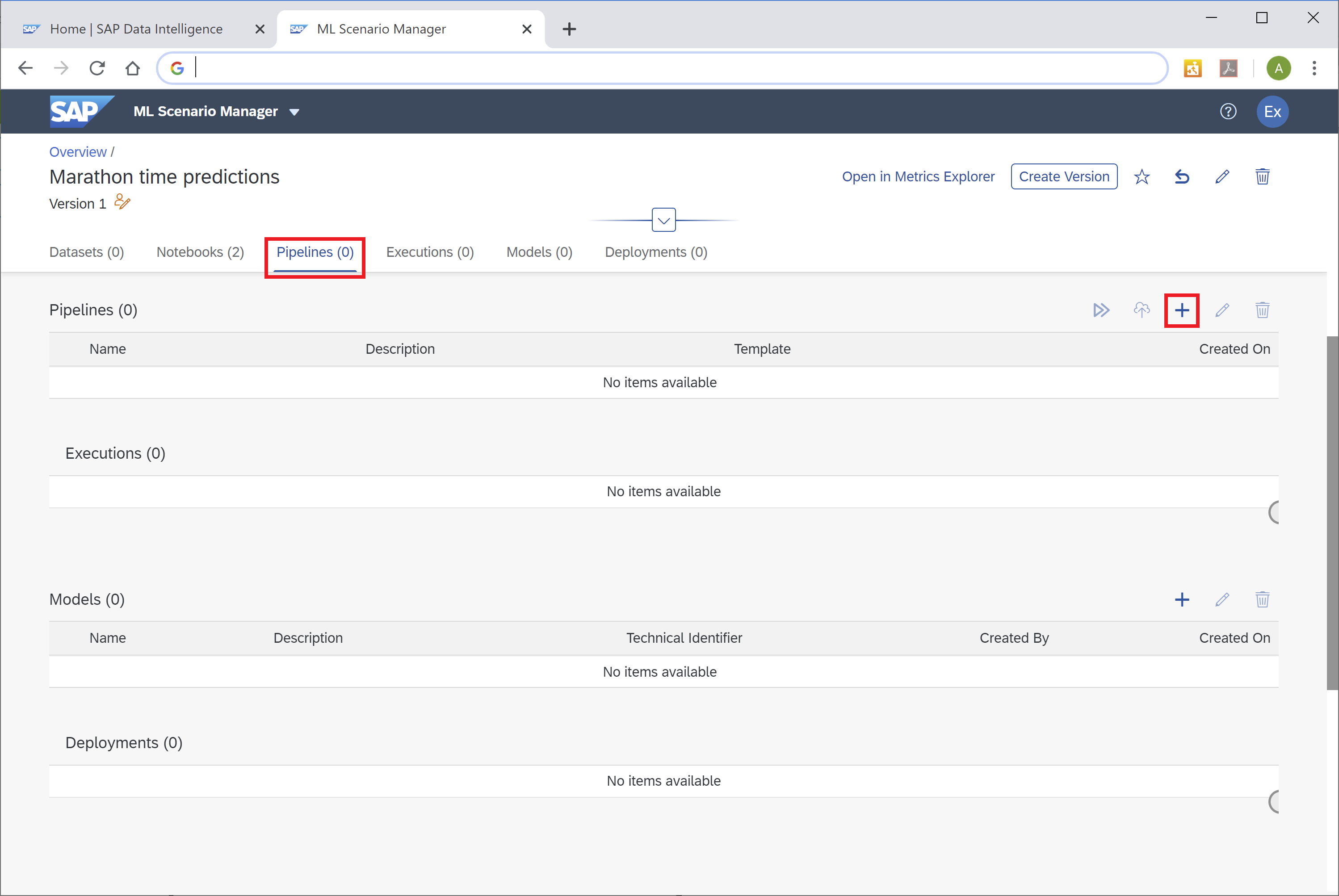
Now start work on the Machine Learning project. On the main page of SAP Data Intelligence click into the "ML Scenario Manager", where you will carry out all Machine Learning related activities.
Click the little "+"-sign on the top right to create a new scenario. Name it "Marathon time predictions" and you enter further details into the "Business Question" section. Click "Create".
You see the empty scenario. You will use the Notebooks to explore the data and to script the regression model in Python. Pipelines bring the code into production. Executions of these pipelines will create Machine Learning models, which are then deployed as REST-API for inference.
But one step at a time. Next, you load and explore the data in a Notebook. Select the "Notebooks" tab, then click the "+"-sign. Name the Notebook "10 Data exploration and model training". Click "Create" and the Notebook opens up. You will be prompted for the kernel, keep the default of "Python 3".
Now you are free to script in Python, to explore the data and train the regression model. The central connection to your DI_DATA_LAKE can be leveraged through Python.
The CSV file can then be loaded into a pandas DataFrame. Just make sure that the value assigned to the bucket corresponds with your own bucket name.
Use Python to explore the data. Display the first few rows for example.
Or plot the runners' half-marathon time against the full marathon time.
There is clearly a linear relationship. No surprise, If you can run a marathon fast, you are also likely to be one of the faster half-marathon runners.
Begin by installing the scikit-learn library, which is very popular for Machine Learning in Python on tabular data such as ours.
Then continue by training the linear regression model with the newly installed scikit-learn library. In case you are not familiar with a linear regression, you might enjoy the openSAP course "Introduction to Statistics for Data Science".
Plot the linear relationship that was estimated.
Calculate the Root Mean Squared Error (RMSE) as quality indicator of the model's performance on the training data. This indicator will be shown later on in the ML Scenario Manager.
In this introductory example the RMSE is calculated rather manually. This way, I hope, it easier to understand its meaning, in case you have not yet been familiar with it. Most Data Scientists would probably leverage a Python package to shorten this bit.
A statistician may want to run further tests on the regression, ie on the distribution of the errors. We skip these steps in this example.
You could apply the model immediately on a new observation. However, to deploy the model later on, we will be using one graphical pipeline to train and save the model and a second pipeline for inference.
Hence at this point we also spread the Python code across two separate Notebooks for clarity. Therefore we finish this Notebook by saving the model. The production pipeline will save the model as pickled object. Hence the model is also saved here in the Notebook as pickle object as well.
Don't forget to save the Notebook itself as well.
To create the second Notebook, go back to the overview page of your ML Scenario and click the "+"-sign in the Notebooks section.
Name the new Notebook "20 Apply model", confirm "Python 3" as kernel and the empty Notebook opens up. Use the following code to load the model that has just been saved.
It's time to apply the model. Predict a runner's marathon time if the person runs a half-marathon in 2 hours.
The model estimates a time of just under 4 hours and 24 minutes.
Now everything is in place to start deploying the model in two graphical pipelines.
To create the graphical pipeline to retrain the model, go to your ML Scenario's main page, select the "Pipelines" tab and click the "+"-sign.
Name the pipeline "10 Train" and select the "Python Producer"-template.

You should see the following pipeline, which we just need to adjust. In principle, the pipeline loads data with the "Read File"-operator. That data is passed to a Python-operator, in which the ML model is trained. The same Python-operator stores the model in the ML Scenario through the "Artifact Producer". The Python-operator's second output can pass a quality metric of the model to the same ML Scenario. Once both model and metric are saved, the pipeline's execution is ended with the "Graph Terminator".
Now adjust the template to our scenario. Begin with the data connection. Select the "Read File"-operator and click the "Open Configuration" option.
In the Configuration panel on the right-hand side open the "Connection"-configuration, set "Configuration type" to "Connection Management" and you can set the "Connection ID" to the "DI_DATA_LAKE.
Save this configuration. Now open the "Path" setting and select the RunningTimes.csv file you had uploaded.
Next we adjust the Python code that trains the regression model. Select the "Python 3"-operator and click the Script-option.
The template code opens up. It shows how to pass the model and metrics into the ML Scenario. Replace the whole code with the following. That code receives the data from the "Read File"-operator, uses the code from the Notebook to train the model and passes the trained model as well as its quality indicator (RMSE) to the ML Scenario.
Close the Script-window, then hit "Save" in the menu bar.
Before running the pipeline, we just need to create a Docker image for the Python operator. This gives the flexibility to leverage virtually any Python library, you just need to provide the Docker file, which installs the necessary libraries. You find the Dockerfiles by clicking into the "Repository"-tab on the left, then right-click the "Dockerfiles" folder and select "Create Docker File".
Name the file python36marathon.

Enter this code into the Docker File window. This code leverages a base image that comes with SAP Data Intelligence and installs the necessary libraries on it. It's advised to specify the versions of the libraries to ensure that new versions of these libraries do not impact your environment.
SAP Data Intelligence uses tags to indicate the content of the Docker File. These tags are used in a graphical pipeline to specify in which Docker image an Operator should run. Open the Configuration panel for the Docker File with the icon on the top-right hand corner.
Add a custom tag to be able to specify that this Docker File is for the Marathon case. Name it "marathontimes". No further tags need to be added, as the base image com.sap.sles.base already contains all other tags that are required ("sles", "python36", "tornado").
The "Configuration" should look like:
Now save the Docker file and click the "Build"-icon to start building the Docker image.

Wait a few minutes and you should receive a confirmation that the build completed successfully.
Now you just need to configure the Python operator, which trains the model, to use this Docker image. Go back to the graphical pipeline "10 Train". Right-click the "Python 3"-operator and select "Group".
Such a group can contain one or more graphical operators. And on this group level you can specify which Docker image should be used. Select the group, which surrounds the "Python 3" Operator. Now in the group's Configuration select the tag "marathontimes". Save the graph.

The pipeline is now complete and we can run it. Go back to the ML Scenario. On the top left you notice a little orange icon, which indicates that the scenario was changed after the current version was created.
Earlier versions of SAP Data Intelligence were only able to execute pipelines that had no changes made to them after the last version was taken. This requirement has been removed, hence there is no need to create a new version at the moment. However, when implementing a productive solution, I strongly suggest to deploy only versioned content.
You can immediately execute this graph, to train and save the model! Select the pipeline in the ML Scenario and click the "Execute" button on the right.
Skip the optional steps until you get to the "Pipeline Parameters". Set "newArtifactName" to lm_model. The trained regression model will be saved under this name.
Click "Save". Wait a few seconds until the pipeline executes and completes. Just refresh the page once in a while and you should see the following screen. The metrics section shows the trained model's quality indicator (RMSE = 16.96) as well as the number of records that were used to train the model (n = 116). The model itself was saved successfully under the name "lm_model".
If you scroll down on the page, you see how the model's metrics as well as the model itself have become part of the ML scenario.
We have our model, now we want to use it for real-time inference.
Go back to the main page of your ML Scenario and create a second pipeline. This pipeline will provide the REST-API to obtain predictions in real-time. Hence call the pipeline "20 Apply REST-API". Now select the template "Python Consumer". This template contains a pipeline that provides a REST-API. We just need to configure it for our model.
The "OpenAPI Servlow" operator provides the REST-API. The "Artifact Consumer" loads the trained model from our ML scenario and the "Python36 - Inference" operator ties the two operators together. It receives the input from the REST-API call (here the half-marathon time) and uses the loaded model to create the prediction, which is then returned by the "OpenAPI Servlow" to the client, which had called the REST-API.
We only need to change the "Python36 - Inference"-operator. Open its "Script" window. At the top of the code, in the on_model() function, replace the single line "model = model_blob" with
Add a variable to store the prediction. Look for the on_input() function and add the line "prediction = None" as shown:
Below the existing comment "# obtain your results" add the syntax to extract the input data (half-marathon time) and to carry out the prediction:
Further at the bottom of the page, change the "if success:" section to:
Close the editor window. Finally, you just need assign the Docker image to the "Python36 - Inference" operator. As before, right-click the operator and select "Group". Add the tag "marathontimes".
Save the changes and go back to the ML Scenario. Now deploy the new pipeline. Select the pipeline "20 Apply REST-API" and click the "Deploy" icon.
Click through the screens until you can select the trained model from a drop-down. Click "Save".
Wait a few seconds and the pipeline is running!
As long as that pipeline is running, you have the REST-API for inference. So let's use it! There are plenty of applications you could use to test the REST_API. My personal preference is Postman, hence the following steps are using Postman. You are free to use any other tool of course.
Copy the deployment URL from the above screen. Do not worry, should you receive a message along the lines of "No service at path XYZ does not exist". This URL is not yet complete, hence the error might come up should you try to call the URL.
Now open Postman and enter the Deployment URL as request URL. Extend the URL with v1/uploadjson/. Change the request type from "GET" to "POST".
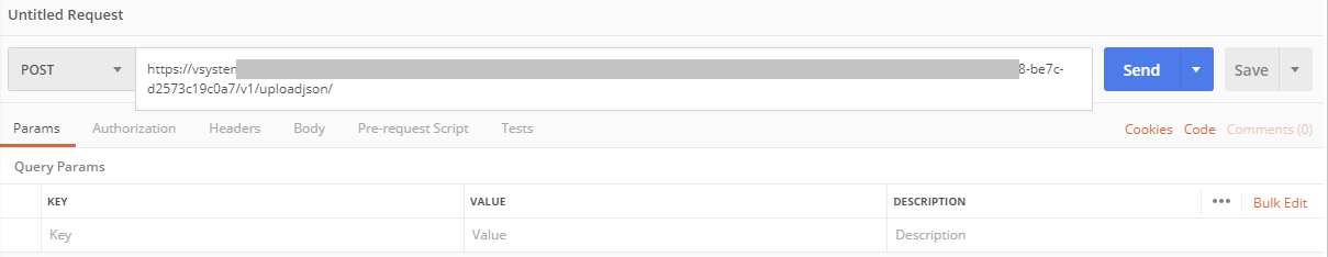
Go to the "Authorization"-tab, select "Basic Auth" and enter your user name and password for SAP Data Intelligence. The user name starts with your tenant's name, followed by a backslash and your actual user name.

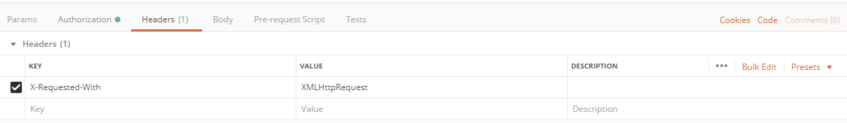
Go to the "Headers"-tab and enter the key "X-Requested-With" with value "XMLHttpRequest".
Finally, pass the input data to the REST-API. Select the "Body"-tab, choose "raw" and enter this JSON syntax:
Press "Send" and you should see the prediction that comes from SAP Data Intelligence! Should you run a half-marathon in 2 hours, the model estimates a marathon time of under 2 hours 24 minutes. Try the REST-API with different values to see how the predictions change. Just don't extrapolate, stay within the half-marathon times of the training data.

Should you prefer to authenticate against the REST-API with a certificate, instead of a password, then see Certificate Authentication to call an OpenAPI Servlow pipeline on SAP Data Intelligence.
You have used Python in Jupyter Notebooks to train a Machine Learning model and the code has been deployed in a graphical pipeline for productive use. Your business processes and application can now leverage these predictions. The business users who benefit from these predictions, are typically not exposed to the underlying technologies. They should just receive the information they need, where and when they need it.
Let me give an example that is more business related than running times. Here is a screenshot of a Conversational AI chatbot, which uses such a REST-API from SAP Data Intelligence to estimate the price of a vehicle. The end users is having a chat with a bot and just needs to provide the relevant information about a car to receive a price estimate.

Happy predicting!
If you liked this exercise and you want to keep going, you could follow the next blog, which uses SAP Data Intelligence to train a Machine Learning model inside SAP HANA, using the Machine Learning that is embedded inside SAP HANA:
SAP Data Intelligence: Deploy your first HANA ML pipelines
In case you want to stick with native Python, you may wonder how to apply the concept from this blog with your own, more realistic, dataset, that contains more than a single predictor. Below are the most import differences for using three predictors instead of just one. In this new example, we predict the price of a used vehicle, using the car's mileage, horse power, and the year in which the car was build.
Training the model in Jupyter:
Applying the model in Jupyter:
Training the model in the pipeline. Just as in Jupyter:
Inference pipeline, retrieving the new predictor values and creating the new prediction:
Inference pipeline, returning the prediction:
Passing the values from Postman:
This blog shows how to create a very basic ML project in SAP Data Intelligence, We will train a linear regression model in Python with just a single predictor column. Based on how many minutes it takes a person run a half-marathon, the model will estimate the person's marathon time. That trained model will then be exposed as REST-API for inference. Your business applications could now leverage these predictions in your day-to-day processes. After this introductory tutorial you will be familiar with the core components of an ML scenario in SAP Data Intelligence, and the implementation of more advanced requirements is likely to follow a similar pattern.
For those who prefer R instead of Python, Ingo Peter has published a blog which implements this first ML Scenario with R.
Should you have access to a system you can follow hands-on yourself. You can currently request a trial or talk to your Account Executive anytime.
Update on 3 April 2023:
- Please note that SAP Data Intelligence is not intended as one-stop-shop Data Science Platform.
- Recently an issue caused the "Python Producer" and "Python Consumer" template pipelines to disappear. See SAP Note 3316646 to rectify.
- This blog was created with Python 3.6, which isn't supported anymore. See the comment below by tarek.abou-warda on using Python 3.9 instead.
- Examples on using the embedded Machine Learning in SAP HANA, SAP HANA Cloud and SAP Datasphere from SAP Data Intelligence are given in the book "Data Science mit SAP HANA" (that book exists only in German, unfortunately there is no English edition)
Table of contents
- Training data
- Data connection
- Data exploration and free-style Data Science
- Deployment
- Summary
- Looking for more?
Training data
Our dataset is a small CSV file, which contains the running times (in minutes) of 117 people, who ran both the Zurich Marathon as well as a local Half-Marathon in the same region, the Greifenseelauf. The first rows show the fastest runners:
| ID | HALFMARATHON_MINUTES | MARATHON_MINUTES |
| 1 | 73 | 149 |
| 2 | 74 | 154 |
| 3 | 78 | 158 |
| 4 | 73 | 165 |
| 5 | 74 | 172 |
SAP Data Intelligence can connect to range of sources. However, to follow this tutorial hands-on, please place this this file into SAP Data Intelligence's internal DI_DATA_LAKE.
- Open the "Metadata Explorer"
- Select "Browse Connections"
- Click "DI_DATA_LAKE"
- Select "shared" and upload the file
Data connection
Since we are using the built-in DI_DATA_LAKE you do not need any additional connection. If the file was located outside SAP Data Intelligence, then you would create an additional connection in the Connection Management.

If the file was located in an S3 bucket for instance, you would need to create a new connection and and set the "Connection Type" to "S3". Enter the bucket's endpoint, the region and the access key as well as the secret key. Also, set the "Root Path" to the name of your bucket.

Data exploration and free-style Data Science
Now start work on the Machine Learning project. On the main page of SAP Data Intelligence click into the "ML Scenario Manager", where you will carry out all Machine Learning related activities.
Click the little "+"-sign on the top right to create a new scenario. Name it "Marathon time predictions" and you enter further details into the "Business Question" section. Click "Create".

You see the empty scenario. You will use the Notebooks to explore the data and to script the regression model in Python. Pipelines bring the code into production. Executions of these pipelines will create Machine Learning models, which are then deployed as REST-API for inference.

But one step at a time. Next, you load and explore the data in a Notebook. Select the "Notebooks" tab, then click the "+"-sign. Name the Notebook "10 Data exploration and model training". Click "Create" and the Notebook opens up. You will be prompted for the kernel, keep the default of "Python 3".

Now you are free to script in Python, to explore the data and train the regression model. The central connection to your DI_DATA_LAKE can be leveraged through Python.
from hdfs import InsecureClient

import pandas as pd

client = InsecureClient('http://datalake:50070')
The CSV file can then be loaded into a pandas DataFrame. Just make sure that the value assigned to the bucket corresponds with your own bucket name.
with client.read('/shared/i056450/RunningTimes.csv') as reader:

    df_data = pd.read_csv(reader, delimiter=';')
Use Python to explore the data. Display the first few rows for example.
df_data.head(5)Or plot the runners' half-marathon time against the full marathon time.
x = df_data[["HALFMARATHON_MINUTES"]]

y_true = df_data["MARATHON_MINUTES"]


%matplotlib inline

import matplotlib.pyplot as plot

plot.scatter(x, y_true, color = 'darkblue');

plot.xlabel("Minutes Half-Marathon");

plot.ylabel("Minutes Marathon");
There is clearly a linear relationship. No surprise, If you can run a marathon fast, you are also likely to be one of the faster half-marathon runners.

Train regression model
Begin by installing the scikit-learn library, which is very popular for Machine Learning in Python on tabular data such as ours.
!pip install sklearnThen continue by training the linear regression model with the newly installed scikit-learn library. In case you are not familiar with a linear regression, you might enjoy the openSAP course "Introduction to Statistics for Data Science".
from sklearn.linear_model import LinearRegression

lm = LinearRegression()

lm.fit(x, y_true)
Plot the linear relationship that was estimated.
plot.scatter(x, y_true, color = 'darkblue');

plot.plot(x, lm.predict(x), color = 'red');

plot.xlabel("Actual Minutes Half-Marathon");

plot.ylabel("Actual Minutes Marathon");
Calculate the Root Mean Squared Error (RMSE) as quality indicator of the model's performance on the training data. This indicator will be shown later on in the ML Scenario Manager.
In this introductory example the RMSE is calculated rather manually. This way, I hope, it easier to understand its meaning, in case you have not yet been familiar with it. Most Data Scientists would probably leverage a Python package to shorten this bit.
import numpy as np

y_pred = lm.predict(x)

mse = np.mean((y_pred - y_true)**2)

rmse = np.sqrt(mse)

rmse = round(rmse, 2)

print("RMSE: " , str(rmse))

print("n: ", str(len(x)))
A statistician may want to run further tests on the regression, ie on the distribution of the errors. We skip these steps in this example.
Save regression model
You could apply the model immediately on a new observation. However, to deploy the model later on, we will be using one graphical pipeline to train and save the model and a second pipeline for inference.
Hence at this point we also spread the Python code across two separate Notebooks for clarity. Therefore we finish this Notebook by saving the model. The production pipeline will save the model as pickled object. Hence the model is also saved here in the Notebook as pickle object as well.
import pickle

pickle.dump(lm, open("marathon_lm.pickle.dat", "wb"))
Don't forget to save the Notebook itself as well.
Load and apply regression model
To create the second Notebook, go back to the overview page of your ML Scenario and click the "+"-sign in the Notebooks section.

Name the new Notebook "20 Apply model", confirm "Python 3" as kernel and the empty Notebook opens up. Use the following code to load the model that has just been saved.
import pickle

lm_loaded = pickle.load(open("marathon_lm.pickle.dat", "rb"))
It's time to apply the model. Predict a runner's marathon time if the person runs a half-marathon in 2 hours.
x_new = 120

predictions = lm_loaded.predict([[x_new]])

round(predictions[0], 2)
The model estimates a time of just under 4 hours and 24 minutes.

Deployment
Now everything is in place to start deploying the model in two graphical pipelines.
- One pipeline to train the model and save it into the ML Scenario.
- And Another pipeline to surface the model as REST-API for inference
Training pipeline
To create the graphical pipeline to retrain the model, go to your ML Scenario's main page, select the "Pipelines" tab and click the "+"-sign.
Name the pipeline "10 Train" and select the "Python Producer"-template.
You should see the following pipeline, which we just need to adjust. In principle, the pipeline loads data with the "Read File"-operator. That data is passed to a Python-operator, in which the ML model is trained. The same Python-operator stores the model in the ML Scenario through the "Artifact Producer". The Python-operator's second output can pass a quality metric of the model to the same ML Scenario. Once both model and metric are saved, the pipeline's execution is ended with the "Graph Terminator".

Now adjust the template to our scenario. Begin with the data connection. Select the "Read File"-operator and click the "Open Configuration" option.

In the Configuration panel on the right-hand side open the "Connection"-configuration, set "Configuration type" to "Connection Management" and you can set the "Connection ID" to the "DI_DATA_LAKE.

Save this configuration. Now open the "Path" setting and select the RunningTimes.csv file you had uploaded.

Next we adjust the Python code that trains the regression model. Select the "Python 3"-operator and click the Script-option.

The template code opens up. It shows how to pass the model and metrics into the ML Scenario. Replace the whole code with the following. That code receives the data from the "Read File"-operator, uses the code from the Notebook to train the model and passes the trained model as well as its quality indicator (RMSE) to the ML Scenario.
# Example Python script to perform training on input data & generate Metrics & Model Blob

def on_input(data):


    # Obtain data

    import pandas as pd

    import io

    df_data = pd.read_csv(io.StringIO(data), sep=";")


    # Get predictor and target

    x = df_data[["HALFMARATHON_MINUTES"]]

    y_true = df_data["MARATHON_MINUTES"]


    # Train regression

    from sklearn.linear_model import LinearRegression

    lm = LinearRegression()

    lm.fit(x, y_true)


    # Model quality

    import numpy as np

    y_pred = lm.predict(x)

    mse = np.mean((y_pred - y_true)**2)

    rmse = np.sqrt(mse)

    rmse = round(rmse, 2)


    # to send metrics to the Submit Metrics operator, create a Python dictionary of key-value pairs

    metrics_dict = {"RMSE": str(rmse), "n": str(len(df_data))}


    # send the metrics to the output port - Submit Metrics operator will use this to persist the metrics

    api.send("metrics", api.Message(metrics_dict))


    # create & send the model blob to the output port - Artifact Producer operator will use this to persist the model and create an artifact ID

    import pickle

    model_blob = pickle.dumps(lm)

    api.send("modelBlob", model_blob)


api.set_port_callback("input", on_input)
Close the Script-window, then hit "Save" in the menu bar.
![]()
Before running the pipeline, we just need to create a Docker image for the Python operator. This gives the flexibility to leverage virtually any Python library, you just need to provide the Docker file, which installs the necessary libraries. You find the Dockerfiles by clicking into the "Repository"-tab on the left, then right-click the "Dockerfiles" folder and select "Create Docker File".

Name the file python36marathon.
Enter this code into the Docker File window. This code leverages a base image that comes with SAP Data Intelligence and installs the necessary libraries on it. It's advised to specify the versions of the libraries to ensure that new versions of these libraries do not impact your environment.
FROM $com.sap.sles.base

RUN pip3.6 install --user numpy==1.16.4

RUN pip3.6 install --user pandas==0.24.0

RUN pip3.6 install --user sklearn
SAP Data Intelligence uses tags to indicate the content of the Docker File. These tags are used in a graphical pipeline to specify in which Docker image an Operator should run. Open the Configuration panel for the Docker File with the icon on the top-right hand corner.

Add a custom tag to be able to specify that this Docker File is for the Marathon case. Name it "marathontimes". No further tags need to be added, as the base image com.sap.sles.base already contains all other tags that are required ("sles", "python36", "tornado").
The "Configuration" should look like:

Now save the Docker file and click the "Build"-icon to start building the Docker image.
Wait a few minutes and you should receive a confirmation that the build completed successfully.

Now you just need to configure the Python operator, which trains the model, to use this Docker image. Go back to the graphical pipeline "10 Train". Right-click the "Python 3"-operator and select "Group".

Such a group can contain one or more graphical operators. And on this group level you can specify which Docker image should be used. Select the group, which surrounds the "Python 3" Operator. Now in the group's Configuration select the tag "marathontimes". Save the graph.
The pipeline is now complete and we can run it. Go back to the ML Scenario. On the top left you notice a little orange icon, which indicates that the scenario was changed after the current version was created.

Earlier versions of SAP Data Intelligence were only able to execute pipelines that had no changes made to them after the last version was taken. This requirement has been removed, hence there is no need to create a new version at the moment. However, when implementing a productive solution, I strongly suggest to deploy only versioned content.
You can immediately execute this graph, to train and save the model! Select the pipeline in the ML Scenario and click the "Execute" button on the right.

Skip the optional steps until you get to the "Pipeline Parameters". Set "newArtifactName" to lm_model. The trained regression model will be saved under this name.

Click "Save". Wait a few seconds until the pipeline executes and completes. Just refresh the page once in a while and you should see the following screen. The metrics section shows the trained model's quality indicator (RMSE = 16.96) as well as the number of records that were used to train the model (n = 116). The model itself was saved successfully under the name "lm_model".

If you scroll down on the page, you see how the model's metrics as well as the model itself have become part of the ML scenario.

We have our model, now we want to use it for real-time inference.
Prediction / Inference with REST-API
Go back to the main page of your ML Scenario and create a second pipeline. This pipeline will provide the REST-API to obtain predictions in real-time. Hence call the pipeline "20 Apply REST-API". Now select the template "Python Consumer". This template contains a pipeline that provides a REST-API. We just need to configure it for our model.

The "OpenAPI Servlow" operator provides the REST-API. The "Artifact Consumer" loads the trained model from our ML scenario and the "Python36 - Inference" operator ties the two operators together. It receives the input from the REST-API call (here the half-marathon time) and uses the loaded model to create the prediction, which is then returned by the "OpenAPI Servlow" to the client, which had called the REST-API.

We only need to change the "Python36 - Inference"-operator. Open its "Script" window. At the top of the code, in the on_model() function, replace the single line "model = model_blob" with
import pickle

model = pickle.loads(model_blob)
Add a variable to store the prediction. Look for the on_input() function and add the line "prediction = None" as shown:
def on_input(msg):

    error_message = ""

    success = False

    prediction = None # This line needs to be added
Below the existing comment "# obtain your results" add the syntax to extract the input data (half-marathon time) and to carry out the prediction:
# obtain your results

hm_minutes = json.loads(user_data)['half_marathon_minutes']

prediction = model.predict([[hm_minutes]])
Further at the bottom of the page, change the "if success:" section to:
if success:

    # apply carried out successfully, send a response to the user

    msg.body = json.dumps({'marathon_minutes_prediction': round(prediction[0], 1)})
Close the editor window. Finally, you just need assign the Docker image to the "Python36 - Inference" operator. As before, right-click the operator and select "Group". Add the tag "marathontimes".

Save the changes and go back to the ML Scenario. Now deploy the new pipeline. Select the pipeline "20 Apply REST-API" and click the "Deploy" icon.

Click through the screens until you can select the trained model from a drop-down. Click "Save".

Wait a few seconds and the pipeline is running!

As long as that pipeline is running, you have the REST-API for inference. So let's use it! There are plenty of applications you could use to test the REST_API. My personal preference is Postman, hence the following steps are using Postman. You are free to use any other tool of course.
Copy the deployment URL from the above screen. Do not worry, should you receive a message along the lines of "No service at path XYZ does not exist". This URL is not yet complete, hence the error might come up should you try to call the URL.
Now open Postman and enter the Deployment URL as request URL. Extend the URL with v1/uploadjson/. Change the request type from "GET" to "POST".
Go to the "Authorization"-tab, select "Basic Auth" and enter your user name and password for SAP Data Intelligence. The user name starts with your tenant's name, followed by a backslash and your actual user name.
Go to the "Headers"-tab and enter the key "X-Requested-With" with value "XMLHttpRequest".
Finally, pass the input data to the REST-API. Select the "Body"-tab, choose "raw" and enter this JSON syntax:
{

    "half_marathon_minutes": 120

}
Press "Send" and you should see the prediction that comes from SAP Data Intelligence! Should you run a half-marathon in 2 hours, the model estimates a marathon time of under 2 hours 24 minutes. Try the REST-API with different values to see how the predictions change. Just don't extrapolate, stay within the half-marathon times of the training data.
Should you prefer to authenticate against the REST-API with a certificate, instead of a password, then see Certificate Authentication to call an OpenAPI Servlow pipeline on SAP Data Intelligence.
Summary
You have used Python in Jupyter Notebooks to train a Machine Learning model and the code has been deployed in a graphical pipeline for productive use. Your business processes and application can now leverage these predictions. The business users who benefit from these predictions, are typically not exposed to the underlying technologies. They should just receive the information they need, where and when they need it.
Let me give an example that is more business related than running times. Here is a screenshot of a Conversational AI chatbot, which uses such a REST-API from SAP Data Intelligence to estimate the price of a vehicle. The end users is having a chat with a bot and just needs to provide the relevant information about a car to receive a price estimate.
Happy predicting!
Looking for more?
If you liked this exercise and you want to keep going, you could follow the next blog, which uses SAP Data Intelligence to train a Machine Learning model inside SAP HANA, using the Machine Learning that is embedded inside SAP HANA:
SAP Data Intelligence: Deploy your first HANA ML pipelines
In case you want to stick with native Python, you may wonder how to apply the concept from this blog with your own, more realistic, dataset, that contains more than a single predictor. Below are the most import differences for using three predictors instead of just one. In this new example, we predict the price of a used vehicle, using the car's mileage, horse power, and the year in which the car was build.
Training the model in Jupyter:
from sklearn.linear_model import LinearRegression

x = df_data[['YEAR', 'HP', 'KILOMETER']]

y_true = df_data[['PRICE']]

lm = LinearRegression()

lm.fit(x, y_true)
Applying the model in Jupyter:
x_new = [[2005, 150, 50000]]

predictions = lm_loaded.predict(x_new)

round(predictions[0][0], 2)
Training the model in the pipeline. Just as in Jupyter:
    x = df_data[['YEAR', 'HP', 'KILOMETER']]

    y_true = df_data[['PRICE']]
Inference pipeline, retrieving the new predictor values and creating the new prediction:
                input_year = json.loads(user_data)['YEAR']

                input_hp = json.loads(user_data)['HP']

                input_kilometer = json.loads(user_data)['KILOMETER']

                prediction = model.predict([[input_year, input_hp, input_kilometer]])
Inference pipeline, returning the prediction:
msg.body = json.dumps({'car_price': round(prediction[0][0], 2)})Passing the values from Postman:
{

    "YEAR": 2005,

    "HP": 200,

    "KILOMETER": 50000

}- SAP Managed Tags:
- Machine Learning,
- SAP Data Intelligence
Labels:
117 Comments
- « Previous
-
- 1
- 2
- 3
- Next »
You must be a registered user to add a comment. If you've already registered, sign in. Otherwise, register and sign in.
Labels in this area
-
ABAP CDS Views - CDC (Change Data Capture)
2 -
AI
1 -
Analyze Workload Data
1 -
BTP
1 -
Business and IT Integration
2 -
Business application stu
1 -
Business Technology Platform
1 -
Business Trends
1,658 -
Business Trends
91 -
CAP
1 -
cf
1 -
Cloud Foundry
1 -
Confluent
1 -
Customer COE Basics and Fundamentals
1 -
Customer COE Latest and Greatest
3 -
Customer Data Browser app
1 -
Data Analysis Tool
1 -
data migration
1 -
data transfer
1 -
Datasphere
2 -
Event Information
1,400 -
Event Information
66 -
Expert
1 -
Expert Insights
177 -
Expert Insights
294 -
General
1 -
Google cloud
1 -
Google Next'24
1 -
Kafka
1 -
Life at SAP
780 -
Life at SAP
13 -
Migrate your Data App
1 -
MTA
1 -
Network Performance Analysis
1 -
NodeJS
1 -
PDF
1 -
POC
1 -
Product Updates
4,577 -
Product Updates
341 -
Replication Flow
1 -
RisewithSAP
1 -
SAP BTP
1 -
SAP BTP Cloud Foundry
1 -
SAP Cloud ALM
1 -
SAP Cloud Application Programming Model
1 -
SAP Datasphere
2 -
SAP S4HANA Cloud
1 -
SAP S4HANA Migration Cockpit
1 -
Technology Updates
6,873 -
Technology Updates
420 -
Workload Fluctuations
1
Related Content
- Exploring Integration Options in SAP Datasphere with the focus on using SAP extractors - Part II in Technology Blogs by SAP
- Onboarding Users in SAP Quality Issue Resolution in Technology Blogs by SAP
- Improvising Time Management in SAP S/4HANA Cloud: A Co-Innovation Solution in Technology Blogs by SAP
- ABAP RAP - Managed scenario - Create Supplier invoice by Action using EML and I_SUPPLIERINVOICETP in Technology Q&A
- ABAP Cloud Developer Trial 2022 Available Now in Technology Blogs by SAP
Top kudoed authors
| User | Count |
|---|---|
| 35 | |
| 25 | |
| 14 | |
| 13 | |
| 7 | |
| 7 | |
| 6 | |
| 6 | |
| 5 | |
| 5 |