

- SAP Community
- Products and Technology
- Technology
- Technology Blogs by SAP
- Machine Learning with SAP HANA – from R
Technology Blogs by SAP
Learn how to extend and personalize SAP applications. Follow the SAP technology blog for insights into SAP BTP, ABAP, SAP Analytics Cloud, SAP HANA, and more.
Turn on suggestions
Auto-suggest helps you quickly narrow down your search results by suggesting possible matches as you type.
Showing results for
former_member18
Participant
Options
- Subscribe to RSS Feed
- Mark as New
- Mark as Read
- Bookmark
- Subscribe
- Printer Friendly Page
- Report Inappropriate Content
04-09-2019
9:01 AM
In this blog I will show how to build machine learning models in Rstudio and run the training directly in SAP HANA.
The main benefit with this approach is that it allows you to utilize the power of SAP HANA both in terms of scalability and performance through R scripts.
In a nutshell, there is no movement of training data from SAP HANA to the R server/client. With this functionality SAP previously released the Python API that also gave users the ability to interact with SAP HANAs Predictive Analysis Library from their preferred Python GUI like Jupyter, Spyder etc. (see reference list below for links). With the release of HANA.ML.R it is now possible to use R together with SAP HANA - which is something I personally have been looking forward to.
From my own experience as an external SAP Data Science consultant, I see many users prefer R or Python over SQL (Structured Query Language) or SQL Procedures to interact with SAP HANA and SAP HANA PAL.
The data scientist uses the familiar R command interface to invoke algorithms directly in SAP HANA PAL. The CPUs processing required during training of machine learning models is performed on SAP HANA and not on a limited laptop etc. This leverages the performance of SAP HANA and greatly improves the training time of machine learning models.
In this blog, I will show how to build a machine learning model from RStudio or your preferred R GUI on SAP HANA without moving the training data to the R client. This allows as mentioned for faster machine learning training time as SAP HANA is much more performant than a laptop or similar.
Contents:
- Machine learning with SAP HANA - all Interaction performed directly from R.
- Realistic business problem solved with machine learning.
- Appendix. Pre-requisites for using the R Client API for machine learning algorithms with SAP HANA
Firstly I want to showcase how to build a simple machine learning model in SAP HANA - but using the data science language R. SAP HANA comes with a wide set of machine learning algorithms to deal with regression, classification, forecasting etc. This library is called PAL - short for Predictive Analysis Library (see more in the references below). Some of the algorithms in PAL can now be accessed through the use of R. In the following I am using Rstudio as my preferred graphical user interfase to R.
The data that is used in this blog comes from the CoIL (Computational Intelligence and Learning, see link to references) challenge, which had the following goal:
“Can you predict who would be interested in buying
a caravan insurance policy and give an explanation of why?”
The data file features the actual dataset from an insurance company and it contains 5822 customer records of which 348, about 6%, had caravan policies. Each record consists of 86 attributes, containing socio-demographic data product ownership. The test or validation set contained information on 4000 customers randomly drawn from the same population. For model comparison purposes each model must be evaluated as to which of the 800 customers would be most likely to buy caravan policies. Meaning that when scoring a model the highest 20% (800 customers of in total 4000 in the test set) customers must be presented and evaluated for a true prediction.
Selecting the 800 customers randomly would in average only produce 48 customers that would be buying. The competition had two objectives the first being to build a model that could predict most customers from the 800 highest probable customers in the testing dataset.
The dataset is in my view a more realistic as it contains imbalanced classes (only 6% are interested in the product). In this machine learning use case I will show how to use SAP HANAs machine learning library - Predictive Analysis Library to solve this data science challenge. The data is available so if you want to re-produce it should be straight forward.

Building and training machine learning models from R - but on SAP HANA.
Below you see the simple R code needed to train a machine learning model on SAP HANA from Rstudio. In this example, I am using supervised classification algorithms which from my experience performs very well but in terms of training time and generalizing on new data without overfitting. For those who know the R language, this would be very familiar with building machine learning models using packages such as caret (Caret is short for Classification And REgression Training) or mlbench (Machine Learning Benchmark).
Initial R code connecting to your SAP HANA tables.

There are as shown just a few lines of code needed to ask SAP HANA to train a machine learning model from R.
Firstly loading the R library "hana.ml.r". This command also loads additional libraries that are used together with hana.ml.r. Such as RODBC that communicates with SAP HANA. You must ensure that the dependencies are installed in your local R environment.
Secondly connecting to SAP HANA using the hanaml.ConnectionContext function. Here you supply the necessary ODBC link name and your credentials. It is also possible to use the SAP HANA tool hdbuserstore.exe to set your credentials so you won't have to store it in clear text. Run the following command: hdbuserstore.exe set <key> <server> : <port> @ <database> <user> <password>.
Lastly, you use the function conn$table to create a link to the SAP HANA table. Note that this does not transfer the data to R! This is one of the major advantages of using this approach. Also, I create the featurelist and the label name. This could also be set directly in the algorithm function, however for simplicity I chose this method.
Understanding your data:

Using this command R will ask SAP HANA to count the number of rows and only return the result.
Creating a few helper variables:
featurelist <- list("Customer_Subtype" , "Number_of_houses"... )
label <- "Number_of_mobile_home_policies_num"
Now you are ready to ask SAP HANA to train the machine learning models and chose the model that shows the most promising results on unseen data.

In this case i use the random forest algorithm to classify who would be interested in buying the additional insurance product. All classification models are able to execute and predict customers who will be interested in buying the additional insurance product. The algorithm that predicts most customers from the selected 800 most likely customers is from a data science point of view not surprisingly the random forest algorithm. Random Forest has many advantages over single decision tree. Random Forests is an ensemble classifier which uses many decision tree models to predict the result.
model <- hanaml.RandomForestClassifier(conn.context = conn, df = train, features = featurelist, label = label)
Using RStudio you can click tabulator(TAB)-key to see all the possible parameters that the function accepts:

After executing the code line SAP HANA will start the training part and still no data will be transferred to R. All processing will be performed on SAP HANA.
Plotting the number of random forest trees against error (out of bag error):
plot(model$oob.error$Collect())

The chart above illustrates the whether the model keeps improving with more trees using the out of bag error metric. As shown the improvement flattens out after approx 50 trees.
Evaluating the trained model on new data:
Once the model has been trained it can be applied to new (unknown to the model) data.
# Model evaluation
model$confusion.matrix_
ACTUAL_CLASS PREDICTED_CLASS COUNT
1 0 0 5474
2 0 1 0
3 1 0 348
4 1 1 0
The training evaluation metric is accuracy which also reflects in the result. The result might seem terrible, however as mentioned the data is highly imbalanced and as such we could benefit from evaluation metrics like kappa or MCC - I will show how this can be mitigated later in the blog.
For now, I will apply the test data provided with the data science challenge to the very simple model we have built. 1 = the customers that we predicted correctly (out of the possible 238 when choosing the most probable from 800).
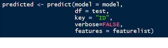
Firstly I create a table link to the SAP HANA table containing the test data. Then I use the predict function to apply the data to the trained model (called "model").
With these simple pieces of code where the most code was getting the data in order to answer the data science challenge. In our case, we can find 103 of the potential 238 customers willing to buy the additional insurance product. If we looked at the leaderboard for the data science challenge this would give us the following place. Choosing randomly one would be able to predict approximately 48 customers (we randomly chose 800 or 20% of 238 actual buying customers ~ 47,6 customers).
Improving our model:
As mentioned above the data science challenge I am using contains a highly imbalanced dataset. In the following I will show how we can improve our model - still keeping the code rather simple and production ready.

With these parameters that now take into account the stratified sampling and prior probabilities for the imbalanced classes we can achieve 110 correct classified customers that would be interested in buying the insurance product. Increasing the number of ensemble trees and also the number of max.depth and max.features also could increase the model a bit further. However in this example I wanted to show the simplicity of R with SAP HANA and not go overboard in code complexity.
Predicting on test data:
Viewing a few records of the predicted table. The field Score is the class (1=buy, 0=no interested) or the model decision and Confidence is how probable the model is of this decision.

Answering the Challenge - the most likely customers to buy the caravan insurance:

This would then bring us to the top 5 - with minimum coding effort and high transparency. Previously I have built an ensemble of 3 machine learning models (random forest, logistic regression, and automated analytics) that correctly predicted 121 customers, however that included lots of coding and it was harder to bring to a potential production stage.
In the data science challenge, there was an additional question besides predicting the most likely customers to buy the new insurance product. Namely answering why these customers would be interested. Below are the few lines of code needed to produce feature importance in descending order:

The most important variables of our study are: Customer_Subtype, Contribution car policies, fire policies and number of cars. This also makes a bit of sense from an insurance business perspective I would expect customer that have one or more cars being more interested in a caravan insurance policy. Without a car it is more unlikely to buy a caravan and hence need a caravan insurance...
Improving predictive capabilities even further:
In a typical data science project, it is essential to prepare the data before addressing which algorithm to use when training a supervised learning model. In the use case above I used the dataset just as they came from the data science challenge. To really squeeze the most possible information out of a dataset it is important to address data preparation even further.
Using the CRiSP-DM implementation approach is normally considered a best practice within the data science community. As explained earlier, the process model consists of different phases as shown below in the figure below.

According to the CRiSP-DM process model the top-level knowledge discovery process consists of business understanding, data understanding, data preparation, modeling, evaluation and deployment. As illustrated, there is an iterative flow between the different phases. See the figure above.
The structure behind the article is to follow the process and methodology quite rigorously so that this can be re-used in other scenarios within predictive analysis. The CRiSP-DM phases of business understanding, data understanding, data preparation, modeling and evaluation are covered in this article, however deployment is deemed outside this scope as it is more a project case-by-case deployed in a custom landscape and more differentiated than the first 5 phases.
Each phase in the methodology contains a number of second-level generic tasks. These second level tasks are defined as generic as they can be used in different data mining situations. Furthermore, these tasks are considered complete and stable, meaning that they cover the whole process of data mining and are valid for unforeseen developments.
The random forest algorithm:
The random forest algorithm is just one of many available algorithms used to solve classification and regression use cases. The random forest algorithm basically optimizes for two parameters.
Firstly the number of features at each split and secondly the number of trees that should be used in the ensemble.
Finding the optimum maximum features (number of variables that should be randomly used for each split) for our model? This can be evaluated using a loop function as shown below:

Plotting the result of max. features (lower values are better):

After 10 randomly chosen variables, the confidence in the model is not hugely changed. It helps to understand here that 10 variables are suitable for the tree split. However, it could also be expanded further. The challenge is here to avoid having the model "remember" all points and in the end overfit. Especially in this use case where our number of transactions is limited to around 6000.
Useful R functions when interacting with SAP HANA:
# Using R to get metadata information about the connected SAP HANA table.
# Counting number of records in table
train$Count()
# Displaying connection parameters
train$connection.context
# Displaying connection schema
train$GetCurrentSchema()
# Counting number of records (same as $Count - I think)
train$nrows
# Generated select statement to SAP HANA DB
train$select.statement
# Columns in connected table
train$columns
# Generate basic statistic on the connected table. Similar to R's summary function.
train$describe()

# Select distinct
train$distinct()
# View data types (integer, nvarchar etc.)
train$dtypes()
Appendix.
Technical setup.
Prerequisites - how to setup the connection between SAP HANA and R.
The HANA ML R package utilizes ODBC (Open Database Connectivity). In order to communicate with SAP HANA from R through the R package "HANA_ML_R". SAP HANA 2.0 SPS04 (released April 5th 2019) is required for the HANA.ml.r package to work. I managed to get most of the functionality running on a SAP HANA 2.0 SPS03, however that is not recommended.
Installing the R package hana.ml.r in your own R environment:
Installing the hana.ml.r package is accomplished like with any other R package that you have locally. Here an example for windows. As of writing this blog the hana.ml.r package is not on CRAN. R >= 3.3.
install.packages("C:/yourdrive/hana.ml.r-1.0.3.tar.gz", repos=NULL, type="source")
When loading the hana.ml.r package it will also import the following packages:
R6, futile.logger, sets, RODBC, uuid
Setting up the ODBC link to SAP HANA:
Step 1: Create an ODBC link to your HANA Server (shown here from Windows)

Step 2:
Add a new ODBC link:

Step 3: Create a new Data Source link with HDBODBC (HANA Database ODBC):

Step 4: Configuring the ODBC link.

Step 5: One important parameter is to make sure that ODBC link is created with the Advanced property as shown below. Without this parameter I have noted strange errors when fetching “lots” of data. The error can be reproduced with a table in SAP HANA with more than ~ 2000 characters accumulated filed names in one table (very normal in customer tables). I think this applies to other databases as well. Luckily there is a simple fix as shown below. This is also described in this blog: https://stackoverflow.com/questions/38969669/why-does-sqlquery-from-sap-hana-using-rodbc-return-no-d...

Step 6: Before trying to use the ODBC link from R make sure it works. Click the Test connection and enter your credentials.

If you get a "Connect successful", you are all good to proceed with the next step where all the fun with machine learning starts.
Accessing more information:
From Rstudio, you can access additional information about the capabilities with the hana.ml.r package.
Help description for the algorithm showcased here.
??hana.ml.r::hanaml.RandomForestClassifier (type this in the R command line or use the GUI to naviate to the help part of RStudio)
Random forest model for classification parameter setup while training:

Available list of algorithms (available as of this writing):

Next step:
In a future blog post, I will show the capabilities of data preparation in more detail from R in SAP HANA - which from a Data Scientists view is an essential task when trying to solve and optimize data science solutions.
Go to part 2:
https://blogs.sap.com/2019/06/07/machine-learning-with-sap-hana-with-r-api.-part-2./
Links to references
- Github - access the scripts and data sources used in this blog. https://github.com/kurtholst/HANA_R_ML
- SAP HANA PAL Documentation – https://help.sap.com/viewer/2cfbc5cf2bc14f028cfbe2a2bba60a50/2.0.03/en-US/c9eeed704f3f4ec39441434db8...
- SAP HANA, express edition documentation: https://help.sap.com/viewer/product/SAP_HANA,_EXPRESS_EDITION/2.0.03/en-US
- SAP HANA, express edition Python Client API for machine learning algorithms documentation: https://help.sap.com/http.svc/rc/869ecfddc30a45868cf47b95760ff5c1/2.0.03/en-US/html/index.html
- Using JupyterLab with HANA: https://blogs.sap.com/2018/10/01/machine-learning-in-a-box-part-10-jupyterlab/
- Installing the Python Client API for machine learning algorithms tutorial: https://developers.sap.com/tutorials/hxe-ua-install-python-ml-api.html
Diving into the HANA DataFrame: Python Integration – Part 1 https://blogs.sap.com/2018/12/17/diving-into-the-hana-dataframe-python-integration-part-1/
- Diving into the HANA DataFrame: Python Integration – Part 2 https://blogs.sap.com/2019/01/28/diving-into-the-hana-dataframe-python-integration-part-2/
- Installing SAP HANA Client tools (ODBC etc.) https://www.youtube.com/watch?v=jfbJ5zc9uJU
- P. van der Putten and M. van Someren (eds). CoIL Challenge 2000: The Insurance Company Case. Published by Sentient Machine Research, Amsterdam. Also a Leiden Institute of Advanced Computer Science Technical Report 2000-09. June 22, 2000. See http://www.liacs.nl/~putten/library/cc2000/
- SAP Managed Tags:
- Machine Learning,
- SAP HANA,
- Big Data,
- SAP Business Technology Platform
Labels:
14 Comments
You must be a registered user to add a comment. If you've already registered, sign in. Otherwise, register and sign in.
Labels in this area
-
ABAP CDS Views - CDC (Change Data Capture)
2 -
AI
1 -
Analyze Workload Data
1 -
BTP
1 -
Business and IT Integration
2 -
Business application stu
1 -
Business Technology Platform
1 -
Business Trends
1,658 -
Business Trends
92 -
CAP
1 -
cf
1 -
Cloud Foundry
1 -
Confluent
1 -
Customer COE Basics and Fundamentals
1 -
Customer COE Latest and Greatest
3 -
Customer Data Browser app
1 -
Data Analysis Tool
1 -
data migration
1 -
data transfer
1 -
Datasphere
2 -
Event Information
1,400 -
Event Information
66 -
Expert
1 -
Expert Insights
177 -
Expert Insights
295 -
General
1 -
Google cloud
1 -
Google Next'24
1 -
Kafka
1 -
Life at SAP
780 -
Life at SAP
13 -
Migrate your Data App
1 -
MTA
1 -
Network Performance Analysis
1 -
NodeJS
1 -
PDF
1 -
POC
1 -
Product Updates
4,577 -
Product Updates
341 -
Replication Flow
1 -
RisewithSAP
1 -
SAP BTP
1 -
SAP BTP Cloud Foundry
1 -
SAP Cloud ALM
1 -
SAP Cloud Application Programming Model
1 -
SAP Datasphere
2 -
SAP S4HANA Cloud
1 -
SAP S4HANA Migration Cockpit
1 -
Technology Updates
6,873 -
Technology Updates
419 -
Workload Fluctuations
1
Related Content
- How to make a REST "PUT" call to a dynamic url and pass Binary file content in body in SAP MDK in Technology Q&A
- Consuming SAP with SAP Build Apps - Mobile Apps for iOS and Android in Technology Blogs by SAP
- App to automatically configure a new ABAP Developer System in Technology Blogs by Members
- Onboarding Users in SAP Quality Issue Resolution in Technology Blogs by SAP
- Embracing TypeScript in SAPUI5 Development in Technology Blogs by Members
Top kudoed authors
| User | Count |
|---|---|
| 36 | |
| 25 | |
| 17 | |
| 13 | |
| 8 | |
| 7 | |
| 6 | |
| 6 | |
| 6 | |
| 6 |