
- SAP Community
- Products and Technology
- Technology
- Technology Blogs by SAP
- Hands-On Tutorial SAP Smart Predict, Customer Chur...
Technology Blogs by SAP
Learn how to extend and personalize SAP applications. Follow the SAP technology blog for insights into SAP BTP, ABAP, SAP Analytics Cloud, SAP HANA, and more.
Turn on suggestions
Auto-suggest helps you quickly narrow down your search results by suggesting possible matches as you type.
Showing results for
Employee
Options
- Subscribe to RSS Feed
- Mark as New
- Mark as Read
- Bookmark
- Subscribe
- Printer Friendly Page
- Report Inappropriate Content
10-31-2018
5:43 AM
Winning back customers who have lost faith in our services or products is a time consuming and costly task. So why not try to prevent customers from seeking their luck elsewhere while they are still customers instead of trying to get them back after they have had (good) experiences with our competition? Wouldn’t it be great if we could identify customers who are at risk of leaving beforehand? Taking actions to prevent them from leaving instead of winning them back with a much bigger effort?
Therefore, customer churn analysis is one of the most popular use cases of predictive analytics. Traditionally this analysis is based on customer data like age, gender and historic sales behavior. Although these are still important customer attributes in times of online shopping we can supplement this with data taken from our online shop like the number of visited pages, the average time spent on our homepage or abandoned shopping cards.
Now that we have seen the importance of customer churn analysis to the business and have identified the data we could use we should try to identify the people who could do such a type of analysis. Does it really need a data scientist - an expensive and scarce resource not available to all companies - for a standard analysis like this, who in turn will not be overly excited by the simplicity of the problem? This is why SAP Analytics Cloud with Smart Predict offers a toolset to the business user that addresses common predictive use cases. With this the business analyst can solve standard statistical use cases on his own, thus freeing the data scientist from routine tasks and provide him more time for doing the heavy lifting.
This guide will walk us through the process of doing a customer churn analysis for online retail shops in SAP Analytics Cloud.
So, let’s have a look at an online shopping portal that sells beauty and pharma products. The collected data describes the usage and activities on the portal. Based on this data we want to predict which customers are most likely to churn. To find patterns in historic data and to train this model the following data set is used:
First, we log on to a SAP analytics Cloud instance.
After the logon the dataset needs to be uploaded. To do this we click on the menu on the left and select “Datasets” and click on “Bring in data from CSV or Excel files”.
On the Pop Up, we select the source file “Customer Churn.csv”, click “Import” and then “Ok”.
Now that we have uploaded the data set we can start to build our predictive scenario. We select “... More” and “Predictive Scenario” on the menu.
A predictive scenario is a set of use cases with common characteristics. SAP Analytic Cloud’s Smart Predict currently offers 3 predictive Scenarios:
The user now has to follow 3 simple steps:
The variable that contains the customer behavior in the learning phase and is predicted in the application phase is called the target variable.
The following screen shot shows the three options classification, regression and time series. Under each option there is a description to make it easier for the user to select the right scenario for each use case. In this exercise, we want to create a model to predict which customers are most likely to churn. Based on the descriptions of predictive scenario types, we can see that a classification will be able to address our needs. So, we select “Classification”.
In the Pop Up window, we give the scenario a name, e.g. “Customer Churn”.
Now we can create our Predictive Model.
We will need to select an input dataset for our model. The input data set contains historical data that we use to train the predictive model.
We select the customer churn data from the folder.
Please check that all data types of the variables where recognized correctly like we see in these:


After all column details are defined correctly we need to select the variable roles:
The target variable is the variable that we try to predict after the learning phase. In our example we select the Target Variable as “Contract Activity”.
Variables that have no influence on the target can be excluded from the modeling process. Excluding variable can speed up the execution process but keeping them does not interfere with the modelling process. In our Example Customer ID (since it is randomly chosen for each customer) has no influence on the target and is excludes as shown on the next screen.

However, we must exclude variables that are directly related to the target variables such as transformations of the target variables and variables that contain indirectly the same information as the target variable. For example, if a dataset contains the variable "has churned Yes/No", and a churn date that indicates when the customer has left us or is empty when he is still active.

Then we click “Train” on the bottom right.
During the Training the tool will automatically test and try to reduce the number of variables in the model depending on quality criteria. This selection is done by successive iterations and only the variables that have influence on the target are kept.
After our model was trained we can select version one. We see displayed two performance indicators to describe the quality of the model. The Predictive Power (KI) indicates the proportion of information contained in the target variable that the model and the explanatory variables are able to explain.
The Prediction Confidence (KR) shows the robustness. It signifies the capacity of the model to achieve the same performance when it is applied to a new dataset exhibiting the same characteristics as the training dataset.
This chart shows all variables that the model generation process identified as relevant on the left and orders them by their impact on the target variable.
On the bottom we see the performance curve. The X axis shows a percentage of the initial population; the Y axis represents the percentage positive targets the algorithm detected.
The green curve shows the maximum possible percentage of detected target (obtained by using the target variable itself as a model). For example, if 25% of your population had the target category ”churned”, then the best model would correctly classify all 25% of the churned customers within 25% of the population.
The red curve shows the minimum percentage of detected target (obtained by a random model). By randomly taking 10% of the population, you would identify 10% of the churned customers.
The blue curve shows the percentage of detected target using our model. For example, if we take 10% of the population we detect roughly 75% of the churned customers. The closer the blue line gets to the green line the better is the model. The larger the distance between the red and the blue line the bigger is the lift of the model.

We select “Variable Contribution” on the top left to better understand the impact and the detailed influence the contributing variables have on the target.


After we had a deeper look at the model and were convinced of its quality we now can apply it. We click on the little factory icon on the top left, use “Customer Churn” (the new data) as input data set and choose a name like “CustomerChurnResults” for the output data set. As input variables we select “All Variables” and as prediction we choose "Predictive Category" and “Prediction Probability”.


On the bottom we can see that the model is being applied. When it is finished we have a look at the results.


We navigate to the menu and select “Files”.
We navigate to the folder where we saved our output dataset, click on the dataset and scroll to the far right.
On the far right we see column “decision_rr_Contract_ Activity” that contains the prediction whether the customer will churn or not based on the probability in column “proba_rr_Contract_ Activity” assigned to the customer by the statistical algorithm. The higher the probability the more likely it is that our customers will churn, the lower it is the more likely it is that they are loyal.
While it is great to see each individual customer, it may be easier for us to consume this information through visualizations. For visualizing the result in an SAP Analytics Cloud story, we first need to build a model on the dataset.

We navigate to the menu and select “Modeler” followed by "From a Data Source”.
We navigate to the folder where we saved our output dataset and select the dataset.
Click “Create Model” in the bottom right and select “Create”.

Once our model has been built, we build our story on top of it.
We navigate to the menu and select “Stories” followed by “From a Smart Discovery”.
We want to explore our results and build a story as easy as possible,that is why we selected Smart Discovery.
We choose our result data set.

Now we need to select the variable that we want to build our story around. In our case we want to learn more about our churners, so we select the contract activity.

After this we need to select our baseline and our target group, in this case our target group are the churners.

Under the included columns section in the advanced options we click on “Measures”.

Here we select “KxIndex” and “proba_rr_Contract_Activity” since they have a direct influence on our target so we need to exclude them. This is similar to what we did in the modeling process when we excluded "Customer ID".
This variable will now not be taken into consideration as key influencing factors, but they will still be available as variables, filters etc. in the Dashboard.

Furthermore under the included columns section in the advanced options we click on “Dimension”. and deselect "decision_rr_Contract_Activity".

We click on “Ok” and then on “Run”.

The tool now generated two pages automatically from the data set: one that gives an overview and one with the key influencers of the model. We see that the exclude variables don’t appear as key influence but are still available as filter and measures/dimension in our visualizations on the overview page. Just like we wanted it.
This is a good starting point for a dashboard. On the right we have a filter where we can select the different measures and then the different visualizations automatically adjust to this selection. So we see the influence, distribution etc. for the churners and active customers.

Maybe these two pages don’t address all our needs yet. No problem since SAP Analytics Cloud is also a self service BI tool so we can adjust them. Let’s go to the edit mode by clicking on “edit” on the top right and adjust the graphs and delete them. We can go freestyle and change the dashboard as we want it.

Additionally, we can add further visualization either on the existing pages or on a new page.For this kind of analysis I find it quite handy to have a table with an in-Column-Chart that shows the churn score for each customer. Let’s have a look how to do this. So we make sure we are in the edit mode and we click on the little plus icon that appears via mouse over next to the key influencers tap.

Select “Canvas” and then add a new object as table.

To structure the table, we select “Rows” and then “Customer_id” so that we can analyze the churn score for each customer.

Under “Columns”, we hover on “Account” and move our mouse to the right. We should see that a filter button appears. We select “KxIndex” and other columns we don’t want to have in our table. Then we click “OK”.


We click on the column header “proba_rr_contract_activity” from within the table and we click on the bullseye icon, selecting “In-Column-Chart”.

On the right side we can adjust the look of this chart, we select “Variance Bar”.

We switch the color since the one with the highest probability are most likely to churn so we want them to be visualized in red.

From the right-side toolbar, we click the arrows to sort the table. We select “Value Sorting”. For type, we select “Descending” and for “Related Dimension Account”, we select “probarr_contract_activity”. Then we click “OK”.


After we sorted the customers based on their score we can now prioritize and contact the ones with the highest score first to prevent them from churning maybe with a campaign.
Be creative and add the company logo or adjust the styling to the company’s corporate identity, add more data, nice charts or a RSS feed. Just try it out.
The official SAP analytics Cloud tutorial and the playlist are very helpful.
https://www.sapanalytics.cloud/learning/
https://wiki.scn.sap.com/wiki/display/BOC/SAP+Analytics+Cloud+-+Official+Product+Tutorials
https://www.youtube.com/playlist?list=PLs5htBIwERYWSixKSqQHzndop33aBCz1U
Have fun with doing your own predictions and building nice dashboards.
Therefore, customer churn analysis is one of the most popular use cases of predictive analytics. Traditionally this analysis is based on customer data like age, gender and historic sales behavior. Although these are still important customer attributes in times of online shopping we can supplement this with data taken from our online shop like the number of visited pages, the average time spent on our homepage or abandoned shopping cards.
Now that we have seen the importance of customer churn analysis to the business and have identified the data we could use we should try to identify the people who could do such a type of analysis. Does it really need a data scientist - an expensive and scarce resource not available to all companies - for a standard analysis like this, who in turn will not be overly excited by the simplicity of the problem? This is why SAP Analytics Cloud with Smart Predict offers a toolset to the business user that addresses common predictive use cases. With this the business analyst can solve standard statistical use cases on his own, thus freeing the data scientist from routine tasks and provide him more time for doing the heavy lifting.
This guide will walk us through the process of doing a customer churn analysis for online retail shops in SAP Analytics Cloud.
So, let’s have a look at an online shopping portal that sells beauty and pharma products. The collected data describes the usage and activities on the portal. Based on this data we want to predict which customers are most likely to churn. To find patterns in historic data and to train this model the following data set is used:
| Customer ID | Unique ID for each customer |
| Usage Category (Month) | Number of time the customer used the online shopping portal in the current month |
| Average Usage (Year) | Average Number of time the customer used the online shopping portal in the past year |
| Usage Category (previous Month) | Number of time the customer used the online shopping portal in the previous month |
| Service Type | Flag whether customer has premium or standard service |
| Product Category | Product category the customers’ orders most frequently in this case only pharma or beauty |
| Message Allowance | Flag whether the customers want to receive messages |
| Average Marketing Activity (Bi-yearly) | Average number of marketing activities for customer in the past two years |
| Average Visit Time (min) | Average time the customer spent on the online shopping portal at each visit |
| Pages per Visit | Average number of pages the customer visits on the online shopping portal at each visit |
| Delta Revenue (Previous Month) | Difference from the revenue by this customer in the current month to the revenues in this month |
| Revenue (Current Month) | Revenue by this customer in the current month |
| Service Failure Rate (%) | Percentage of times the customer used the online shopping portal and certain services failed |
| Customer Lifetime (days) | Number of days since the customer registered |
| Product Abandonment | Number of products the customer has put in schopping cart and the abandoned in the last quarter |
| Contract Activity | Flag whether customer has churned or is active. |
First, we log on to a SAP analytics Cloud instance.
After the logon the dataset needs to be uploaded. To do this we click on the menu on the left and select “Datasets” and click on “Bring in data from CSV or Excel files”.

On the Pop Up, we select the source file “Customer Churn.csv”, click “Import” and then “Ok”.
Now that we have uploaded the data set we can start to build our predictive scenario. We select “... More” and “Predictive Scenario” on the menu.

A predictive scenario is a set of use cases with common characteristics. SAP Analytic Cloud’s Smart Predict currently offers 3 predictive Scenarios:
- Classification scenarios predict the value of a (target) variable that can only have two values like yes and no or 0 and 1. Examples for classification scenarios are
- customer churn with the target variable predicting whether a customer will leave or not
- Propensity to buy with the target variable predicting whether a customer will buy a product offered to him or not
- Fraud with the target variable indicating whether a transaction or claim was fraudulent or not
- Regression scenarios predict the numerical value of a target variable depending on variables describing it. Example for regression scenarios are the prediction of
- The number of customers visiting a shop during lunch time
- The revenue of a customer in the next quarter
- The sales price of a used cars
- Time Series scenarios predict the value of a variable over time taking into account further descriptive variables. Examples of time series scenarios are the prediction of
- Revenue for a product line over the next few quarters
- The number of bicycles hired in a city over the next few days
- Travel expenses in the next few months
The user now has to follow 3 simple steps:
- Choose the predictive scenario that matches his use case.
- Train the model with historic data, i.e. use a data set where the customer behavior (has churned or not) is known. The statistical algorithm will “learn” from this data set, i.e. find patterns that characterize a customer who is likely to churn. There should be enough positive cases (i.e. churned customers) in the training data set.
- Apply the model to a new data set, i.e. use a data set where the customer behavior is unknown. The statistical algorithm will apply the patterns learnt in the previous step to the new data and identify the customers who are likely to churn.
The variable that contains the customer behavior in the learning phase and is predicted in the application phase is called the target variable.
The following screen shot shows the three options classification, regression and time series. Under each option there is a description to make it easier for the user to select the right scenario for each use case. In this exercise, we want to create a model to predict which customers are most likely to churn. Based on the descriptions of predictive scenario types, we can see that a classification will be able to address our needs. So, we select “Classification”.

In the Pop Up window, we give the scenario a name, e.g. “Customer Churn”.
Now we can create our Predictive Model.

We will need to select an input dataset for our model. The input data set contains historical data that we use to train the predictive model.
We select the customer churn data from the folder.
After selecting the input data let’s have a look at the variable details. We click on “Edit column details” directly below the field where we selected the input data and check that all data types of variables were correctly identified.

Please check that all data types of the variables where recognized correctly like we see in these:
After all column details are defined correctly we need to select the variable roles:
The target variable is the variable that we try to predict after the learning phase. In our example we select the Target Variable as “Contract Activity”.
Variables that have no influence on the target can be excluded from the modeling process. Excluding variable can speed up the execution process but keeping them does not interfere with the modelling process. In our Example Customer ID (since it is randomly chosen for each customer) has no influence on the target and is excludes as shown on the next screen.
However, we must exclude variables that are directly related to the target variables such as transformations of the target variables and variables that contain indirectly the same information as the target variable. For example, if a dataset contains the variable "has churned Yes/No", and a churn date that indicates when the customer has left us or is empty when he is still active.
Then we click “Train” on the bottom right.
During the Training the tool will automatically test and try to reduce the number of variables in the model depending on quality criteria. This selection is done by successive iterations and only the variables that have influence on the target are kept.
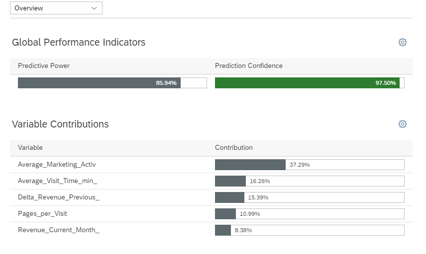
After our model was trained we can select version one. We see displayed two performance indicators to describe the quality of the model. The Predictive Power (KI) indicates the proportion of information contained in the target variable that the model and the explanatory variables are able to explain.
The Prediction Confidence (KR) shows the robustness. It signifies the capacity of the model to achieve the same performance when it is applied to a new dataset exhibiting the same characteristics as the training dataset.
This chart shows all variables that the model generation process identified as relevant on the left and orders them by their impact on the target variable.
On the bottom we see the performance curve. The X axis shows a percentage of the initial population; the Y axis represents the percentage positive targets the algorithm detected.
The green curve shows the maximum possible percentage of detected target (obtained by using the target variable itself as a model). For example, if 25% of your population had the target category ”churned”, then the best model would correctly classify all 25% of the churned customers within 25% of the population.
The red curve shows the minimum percentage of detected target (obtained by a random model). By randomly taking 10% of the population, you would identify 10% of the churned customers.
The blue curve shows the percentage of detected target using our model. For example, if we take 10% of the population we detect roughly 75% of the churned customers. The closer the blue line gets to the green line the better is the model. The larger the distance between the red and the blue line the bigger is the lift of the model.
We select “Variable Contribution” on the top left to better understand the impact and the detailed influence the contributing variables have on the target.
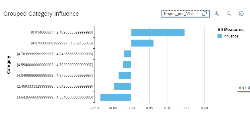
If we select for example “Pages_per_Visit”, we see that the variables have been grouped into values for which the effect on the target is similar, affecting the target in a positive way (more likely to churn on top) or in a negative way (on the bottom).
In our example the customers who seem to be most likely to churn either visit only very few pages – maybe only the home page – or more than 5 pages, whereas customers who only visit 4 to 5 pages seem to be less likely to churn. A possible explanation of this behavior could be that customers who visit only our home page got there by chance or were redirected from elsewhere but are not really interested in our products whereas the customers who had to visit a lot of pages in order to find what they were looking for got frustrated on their way. Looking at the details of variable contribution and trying to explain customer behavior could lead to new business insights.
After we had a deeper look at the model and were convinced of its quality we now can apply it. We click on the little factory icon on the top left, use “Customer Churn” (the new data) as input data set and choose a name like “CustomerChurnResults” for the output data set. As input variables we select “All Variables” and as prediction we choose "Predictive Category" and “Prediction Probability”.
On the bottom we can see that the model is being applied. When it is finished we have a look at the results.
We navigate to the menu and select “Files”.
We navigate to the folder where we saved our output dataset, click on the dataset and scroll to the far right.
On the far right we see column “decision_rr_Contract_ Activity” that contains the prediction whether the customer will churn or not based on the probability in column “proba_rr_Contract_ Activity” assigned to the customer by the statistical algorithm. The higher the probability the more likely it is that our customers will churn, the lower it is the more likely it is that they are loyal.
While it is great to see each individual customer, it may be easier for us to consume this information through visualizations. For visualizing the result in an SAP Analytics Cloud story, we first need to build a model on the dataset.
We navigate to the menu and select “Modeler” followed by "From a Data Source”.

We navigate to the folder where we saved our output dataset and select the dataset.
Click “Create Model” in the bottom right and select “Create”.
Once our model has been built, we build our story on top of it.
We navigate to the menu and select “Stories” followed by “From a Smart Discovery”.

We want to explore our results and build a story as easy as possible,that is why we selected Smart Discovery.
We choose our result data set.
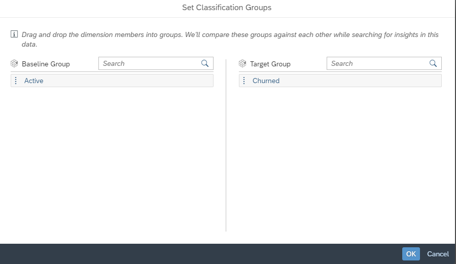
Now we need to select the variable that we want to build our story around. In our case we want to learn more about our churners, so we select the contract activity.
After this we need to select our baseline and our target group, in this case our target group are the churners.
Under the included columns section in the advanced options we click on “Measures”.
Here we select “KxIndex” and “proba_rr_Contract_Activity” since they have a direct influence on our target so we need to exclude them. This is similar to what we did in the modeling process when we excluded "Customer ID".
This variable will now not be taken into consideration as key influencing factors, but they will still be available as variables, filters etc. in the Dashboard.
Furthermore under the included columns section in the advanced options we click on “Dimension”. and deselect "decision_rr_Contract_Activity".
We click on “Ok” and then on “Run”.
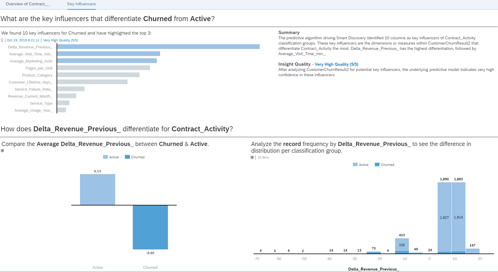
The tool now generated two pages automatically from the data set: one that gives an overview and one with the key influencers of the model. We see that the exclude variables don’t appear as key influence but are still available as filter and measures/dimension in our visualizations on the overview page. Just like we wanted it.
This is a good starting point for a dashboard. On the right we have a filter where we can select the different measures and then the different visualizations automatically adjust to this selection. So we see the influence, distribution etc. for the churners and active customers.
Maybe these two pages don’t address all our needs yet. No problem since SAP Analytics Cloud is also a self service BI tool so we can adjust them. Let’s go to the edit mode by clicking on “edit” on the top right and adjust the graphs and delete them. We can go freestyle and change the dashboard as we want it.
Additionally, we can add further visualization either on the existing pages or on a new page.For this kind of analysis I find it quite handy to have a table with an in-Column-Chart that shows the churn score for each customer. Let’s have a look how to do this. So we make sure we are in the edit mode and we click on the little plus icon that appears via mouse over next to the key influencers tap.
Select “Canvas” and then add a new object as table.
To structure the table, we select “Rows” and then “Customer_id” so that we can analyze the churn score for each customer.
Under “Columns”, we hover on “Account” and move our mouse to the right. We should see that a filter button appears. We select “KxIndex” and other columns we don’t want to have in our table. Then we click “OK”.
We click on the column header “proba_rr_contract_activity” from within the table and we click on the bullseye icon, selecting “In-Column-Chart”.
On the right side we can adjust the look of this chart, we select “Variance Bar”.
We switch the color since the one with the highest probability are most likely to churn so we want them to be visualized in red.
From the right-side toolbar, we click the arrows to sort the table. We select “Value Sorting”. For type, we select “Descending” and for “Related Dimension Account”, we select “probarr_contract_activity”. Then we click “OK”.
After we sorted the customers based on their score we can now prioritize and contact the ones with the highest score first to prevent them from churning maybe with a campaign.
Be creative and add the company logo or adjust the styling to the company’s corporate identity, add more data, nice charts or a RSS feed. Just try it out.
The official SAP analytics Cloud tutorial and the playlist are very helpful.
https://www.sapanalytics.cloud/learning/
https://wiki.scn.sap.com/wiki/display/BOC/SAP+Analytics+Cloud+-+Official+Product+Tutorials
https://www.youtube.com/playlist?list=PLs5htBIwERYWSixKSqQHzndop33aBCz1U
Have fun with doing your own predictions and building nice dashboards.
- SAP Managed Tags:
- SAP Analytics Cloud
Labels:
27 Comments
You must be a registered user to add a comment. If you've already registered, sign in. Otherwise, register and sign in.
Labels in this area
-
ABAP CDS Views - CDC (Change Data Capture)
2 -
AI
1 -
Analyze Workload Data
1 -
BTP
1 -
Business and IT Integration
2 -
Business application stu
1 -
Business Technology Platform
1 -
Business Trends
1,658 -
Business Trends
92 -
CAP
1 -
cf
1 -
Cloud Foundry
1 -
Confluent
1 -
Customer COE Basics and Fundamentals
1 -
Customer COE Latest and Greatest
3 -
Customer Data Browser app
1 -
Data Analysis Tool
1 -
data migration
1 -
data transfer
1 -
Datasphere
2 -
Event Information
1,400 -
Event Information
66 -
Expert
1 -
Expert Insights
177 -
Expert Insights
298 -
General
1 -
Google cloud
1 -
Google Next'24
1 -
Kafka
1 -
Life at SAP
780 -
Life at SAP
13 -
Migrate your Data App
1 -
MTA
1 -
Network Performance Analysis
1 -
NodeJS
1 -
PDF
1 -
POC
1 -
Product Updates
4,577 -
Product Updates
344 -
Replication Flow
1 -
RisewithSAP
1 -
SAP BTP
1 -
SAP BTP Cloud Foundry
1 -
SAP Cloud ALM
1 -
SAP Cloud Application Programming Model
1 -
SAP Datasphere
2 -
SAP S4HANA Cloud
1 -
SAP S4HANA Migration Cockpit
1 -
Technology Updates
6,873 -
Technology Updates
421 -
Workload Fluctuations
1
Related Content
- SAP Signavio is the highest ranked Leader in the SPARK Matrix™ Digital Twin of an Organization (DTO) in Technology Blogs by SAP
- ABAP Cloud Developer Trial 2022 Available Now in Technology Blogs by SAP
- Hack2Build on Business AI – Highlighted Use Cases in Technology Blogs by SAP
- New Machine Learning features in SAP HANA Cloud in Technology Blogs by SAP
- Unify your process and task mining insights: How SAP UEM by Knoa integrates with SAP Signavio in Technology Blogs by SAP
Top kudoed authors
| User | Count |
|---|---|
| 38 | |
| 25 | |
| 17 | |
| 13 | |
| 7 | |
| 7 | |
| 7 | |
| 7 | |
| 6 | |
| 6 |