
- SAP Community
- Products and Technology
- Financial Management
- Financial Management Blogs by SAP
- BPC Planning for S/4HANA – FOX formulas – Part 4
Financial Management Blogs by SAP
Get financial management insights from blog posts by SAP experts. Find and share tips on how to increase efficiency, reduce risk, and optimize working capital.
Turn on suggestions
Auto-suggest helps you quickly narrow down your search results by suggesting possible matches as you type.
Showing results for
Product and Topic Expert
Options
- Subscribe to RSS Feed
- Mark as New
- Mark as Read
- Bookmark
- Subscribe
- Printer Friendly Page
- Report Inappropriate Content
08-21-2018
11:54 AM
Use Case
You would like to learn to program in FOX (formula extension language) to utilise the BPC FORMULA planning functions in BPC Consolidation- or BPC Planning Models.
Content
I started writing a blog on coding FOX formulas and happened to be working on a BPC Optimized for S/4HANA system. My intention was just to write a single blog but found it developing into a few parts due to the length and the fact that I wanted to build the system from scratch, including the entire data model.
So this is PART 4 of a 4-part blog with the following structure:
PART 1 – Setting up the data model, creating an Analysis for Office workbook, capturing and saving some seeding data to the data model. (No fox code yet)
PART 2 – Write a “Hello World” equivalent fox formula and execute it from a button placed in the Analysis for Office workbook.
PART 3 – Tools for debugging functions, variables, constants, loops, If-statements, messages.
PART 4 – Capturing data directly into the cube without using Analysis for Office, "DO" loops, "TMVL()" expression - time value offset calculations, "ATRV()" expression - using attribute values of a dimension member, a complete look at what it takes to calculate production quantities from sales demand and working across 2 cubes, periodic escalations of prices and quantities, overhead costs and cost of sales price calculations, sales price calculation based on a markup percentage, sales income calculation and cost of sales calculations.
Capture data into the cube WITHOUT an input-ready query
In PART 3 we calculated two internal FOX variables and didn't write any data to the cube but in this part we are going to produce a number of output records.
However, let's start by capturing some planning data directly into the cube without using Analysis for Office so we can save some material cost prices for later use in our FOX formulas.
It's a new blog so let's create a new planning function. From Eclipse, NAVIGATE, OEPN SAP GUI, transaction code RSPLAN, select PLANNING FUNCTION, CREATE and complete the pop-up screen as we've done in previous parts but using ID = ZFUNC03, a new description and select the FIELDS TO BE CHANGED as per our part 3.
In the BW PERSPECTIVE of Eclipse we can open the InfoArea on the left and see all the BW objects we've created so far in the various blog parts.
Now select PARAMETER, SAVE the blank screen and exit. We'll come back to the function after we capture some data.

Select PLANNING SEQUENCE, CREATE and complete the ID & Description for a new sequence.

Add the blank function ZFUNC03 to the first sequence step as we've done in the previous parts but now add step 2 as TYPE = 1 Manual Input and the aggregation level and filter are the same ZPAL01 and ZFIL01.

If you now select row 2 and press the EXECUTE button then a cross-tab opens with the filtered data in a ready-for-input state.

From this input cross-tab you are able to VIEW data in your aggregation level + filter, EDIT existing data, ADD new rows and SAVE the additions / changes.

Add 6 new rows to the cross-tab and capture raw material prices for the manufacturing cost centre CC01 for PART01 to PART06. You'll notice since the data is going to be saved to the costing InfoCube ZCST01 the PROFIT CENTER is not valid and we set it to NONE by using the #. We are capturing the cost prices to period 1 as key figure AMOUNT in EUR. SAVE.

Function objectives
Now that we have captured sales quantities and raw material cost prices for period 1 we can derive the rest of the data required to determine sales income. We will make certain assumptions based on the follow data table:
| Period 1 | Sales Qty | Production Qty | Sales Price | Cost Price |
| Drones | 100 | n/a | Markup 40% | RawMats + OH(@15%) |
| Robots | 80 | n/a | Markup 60% | RawMats + OH(@12%) |
| 3D Printers | 150 | n/a | Markup 35% | RawMats + OH(@9%) |
| Rotor blade | n/a | Sales Qty * 80% * 4 | n/a | 52 |
| Drone body | n/a | Sales Qty * 90% | n/a | 837 |
| Robot AI CPU unit | n/a | Sales Qty * 50% | n/a | 3000 |
| Robot body | n/a | Sales Qty * 50% | n/a | 1500 |
| Printer casing | n/a | Sales Qty | n/a | 5000 |
| Printer head | n/a | Sales Qty * | n/a | 2500 |
| Overheads | n/a | n/a | n/a | n/a |
We will start in period 1 with these values and add 2% escalation to sales quantity per month and 3% escalation to raw material prices per month.
We can determine production quantities as a % of sales quantities as we are assuming we hold some stock e.g. if we hold 20% stock of Rotor blades then we only have to produce 80% of the sales quantity demand multiplied by 4 rotor blades per drone and so on for each production item.
For the cost price of the finished goods we will add up the raw material costs and add an amount for overheads at a % of total raw material costs.
For sales price we will markup the finished goods cost price by a certain % e.g. Drones at 40% to total cost price.
Note:
We can also determine sales income for the appropriate GL account, manage the stock levels and post the correct accounting entries but the purpose of this exercise is to demonstrate the use of FOX to perform all these calculations without trying to over-complicate this small piece of demo code. If we wanted a nice report we would extend the data model with a few more key figures for opening- and closing balances, debit- and credit movements and stock locations but we are going to keep things simple and only calculate the most obvious entries and a more complete conceptual data model design can be a topic for another blog.
Step 1: Perform the periodic escalation calculations
1.1 Create a new function
The new function will use the same fields to be changed as the previous functions we have written which are all except 0FISCVARNT, 0FISCYEAR and ZVERSION.

1.2 Declare the local variables
Declare variables for all the characteristics that we will be working with and remember to use the DATA TYPES pop-up to make selections easier.

We want to escalate the first quarter quantities and prices to the rest of the year and we can't use the normal FOREACH loop to do this. See what happens if we try:
We declare a variable V_PER for 0FISCPER3 and then execute a FOREACH loop over it but the result is a loop of the existing 3 values in the fact table i.e. period 1,2 and 3.


1.3 Test the correct functioning of the DO LOOP
So this time we will use the "DO" loop with the "n TIMES" option to loop for 12 times, one for each month / period of the year. Next we use the TMVL (time value) function inside the loop to determine the next period with an offset of 1 and assign it to V_PER. This way we determine independently of the data in the fact table periods 1...12.


1.4 Write the QUANTITY escalation function
Now that we've gained control over the loop for 12 periods we can flesh the function out by adding a variable to keep track of the prior period, V_PPER, so we can escalate the current period up against the prior period. In the DO loop we add an IF statement to perform the escalations only on periods 2 to 12 and you will notice that when using the OPERANDS pop-up helper screen even the local variables declared within the function are identified as VARIABLES that can be selected instead of hard-coded characteristic values i.e. in the example V_PER.
One more thing to notice is that when selecting characteristic values from the drop down list vs typing it in manually the drop-down list will enter the value in the field in the internal format which is correct for the function. As an example if you typed the GL account "1000" it would appear like that in your function but would fail to validate because the required internal format is the one with the leading zeros.

We complete the first of our 2 escalation functions in line 17 and 18 and wrap it in a FOREACH loop to cycle through all profit centres and finished goods items in those profit centres V_PC and V_ITEM. In line 18 we are using the quantity ZQTY from the prior period V_PPER, escalating it and assigning the result to the ZQTY for the current period V_PER in line 17.
You'll see that we hard-coded the 0INFOPROV to ZREV01, our revenue cube, and our cost centre parameter is hard-coded to "#" as this characteristic doesn't exist in this cube. So what would happen if we changed this and captured ZCST01 instead of ZREV01 and left everything else the same? Since ZQTY is a valid key figure of cube ZCST01 the only invalid parameter would be the V_PC profit centre value, so V_PC is ignored and the value is written to the cost cube, ZCST01, with no profit centre as it is not even part of the cube design.
Notice that the escalation % for sales quantity is 2% written as "1.02" but we also need a period "." to complete the coding line so the result is a code line that ends with "...V_PC} * 1.02." When writing expressions with floating point number using a decimal point the system interprets this correctly.
I've also expanded my debugging values by adding line 9 and 24. Line 9 declares a floating point key figure variable and line 24 assigns the last value of the FOREACH loop to it so we can output the value in the MESSAGE statement in line 25 against the last V_PC and V_ITEM values.

If you execute this function now with the TRACE mode in the planning sequence and display the TRACE line items you will see a comprehensive view of the results. At the bottom of the screen in our MESSAGE statements we can see how there are no V_PC and V_ITEM values for V_DBUG01 for period 1. However for period 2, 3, 4 and 5 the results are 153, 156, 159 and 162 which results from (150 * 1.02 = 153), (153 * 1.02 = 156), (156 * 1.02 = 159) and (159 * 1.02 = 162) respectively. These results are seen in much more detail in the TRACE log where not only the last item of the FOREACH loop is seen but all the data with BEFORE, AFTER, REFERENCE and NEW records generated. We can see the 5th period value of 162 for PC03 (V_PC) and PRD03 (V_ITEM).
1.5 Write the COST PRICE escalation business rule (ATTRIBUTE usage)
Now it's time to add the second escalation function to increase raw material prices by 3% each month and we can add it inside the outer periodic DO loop. It's also a good opportunity to demonstrate the use of reading attribute values of a characteristic. So the idea here is to loop through all available material items and only select those that are not finished goods, which we have identified by the attribute ZTYPE set to "FG", and increase those product cost prices.

Before we write the actual escalation function we just want to check that we are identifying the correct ITEMS by their attribute values ZTYPE. We do this by setting up a FOREACH loop around all V_ITEM for each cycle of the period loop. Inside this FOREACH loop we read the attribute value and assign it to a new variable I've named V_ITYPE with the expression ATRV(). The parameters of ATRV() are very simple. The first parameter is the attribute technical name you want to read from the characteristic and in our case we only have one attribute and it's ZTYPE. The second parameter is the characteristic member in the master data that you want to read. In our case it is all materials in our aggregation level sent to the ATRV() expression one at a time by mean of a variable, V_ITEM, in our FOREACH loop.
By outputting the value of the attribute in a MESSAGE statement we can be sure we are identifying the correct materials before we insert our function and delete the MESSAGE statement.

Executing the function in the planning sequence should now output the MESSAGE statement with the PERIOD, ITEM and ATTRIBUTE values. Very often the attribute value is blank the first time you execute this and it is usually as a result of the master data not being activated in RSA1. Find the characteristic ZITEM in RSA1, right-click for context menu and execute ACTIVATE MASTER DATA. Then exit eclipse and logon again to update your session meta-data and you should get the correct result.

The final loop and function are depicted in the screen-shot. In line 22 we have the FOREACH loop around all the materials, V_ITEM, and in line 23 we read each items attribute ZTYPE and use it in line 24 to exclude any item with the attribute set to "FG". All other material items have their cost prices in the costing cube ZCST01 escalated by 3%.

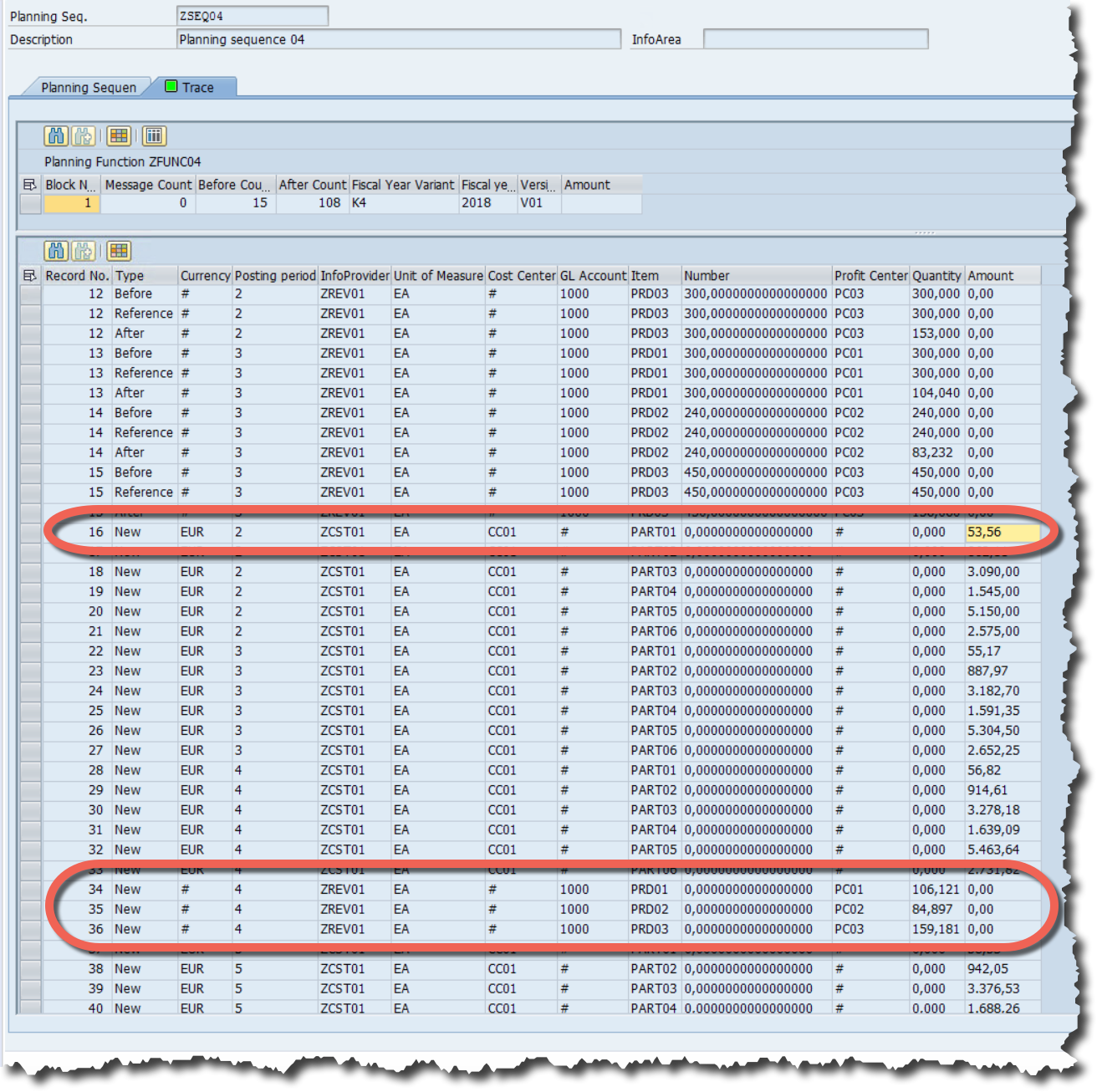
If you execute this code in TRACE mode we can check the results for correctness. We can see in period 1 that the captured price of PART01 is 52. We can also see no other calculation or record was created for period 1 so we know our IF statement is working.

In period 2 and onward we can see that the same item generated a new record and the value is correctly calculated as 52 * 1.03 = 53.56. We can also see that the finished goods materials were excluded from any price calculations. (We will populate these cost prices later as a result of the cumulated raw material prices plus some overhead costs)
1.5 Write the manufacturing and sales business rules
I've added some comments to the current function and in particular the business rules we need to write:
- Calculate the raw material quantities for the period
- Post the raw material purchases GL entries
- Calculate the overhead costs and cost of production
- Post the GL entries and raw material quantities
- Calculate the sales income
- Post GL cost of sales entries

It's also often very useful to declare local variables for the data you are representing in the cube. The variables are easier to read in the code and physically shorter to write. I've declared variables for sales quantity, sales prices, sales cost-of-sales prices, production quantities and raw material prices.

1.5.1 Calculate the raw material quantities for the period
In lines 65 to 74 we set the local variables for sales quantities and raw material prices and in lines 76 to 83 we perform the production quantity calculation, which in our case is a purchasing quantity, based on the assumptions we made in our data table. We then assign the results in lines 85 to 90 from our local variables back to the relevant key figure in the cost cube.
At face value it might seem simpler to ignore the local variables and perform the calculation directly into the cube. There is no right or wrong here and you can do either. The local variable do reduce the risk of mistyping one of the parameters and increase readability but in this simple formula add additional lines to the code.

1.5.2 Post the raw material purchases GL entries
To create the raw material GL postings I've declared a new local variable to hold the result of the GL entry value I want to post and called it V_GLAMT.

Row 94 calculates the GL entry value and stores it in local variable V_GLAMT by multiplying the quantity purchased by the purchase price for the period for each part. Remember purchase quantities are based on the result of the escalating sales quantity and RM prices are escalating periodically so this calculation is done after those two calculations are complete.
The GL entry is done in the costing cube DR RAW MATERIAL GL account and CR ACCOUNTS PAYABLE. The DR and CR entries are indicated by positive and negative values respectively.


1.5.3 Calculate the overhead costs and cost of sales price per unit
At this point we are going to assume the final assembly process takes place and we will simply cost the final products at the current periods RM costs + the assembly overhead.

The overhead calculations are relatively simple in this case as each finished product in the revenue cube ZREV01 is made up of only 2 raw material parts and except for the rotor blades, which use 4 blade per finished good, the rest are all a 1-to-1 ratio. Our overhead calculation is also very simple as we are just increasing the total material price by an overhead percentage. All the calculations are performed using the local variables and then assigned back to the cube to generate data rows at the end of the calculation in line 114-116.

Notice in line 102-104 I added a debug line to view the the raw material prices and quantities as I was getting a small calculation difference on the previous calculation of the accounts payable and found that if was due to rounding as my report I used to re-perform the calculation did not show the decimal places. So you can use an Analysis for Office report, Design Studio cross tab, RSA1 right-click the cube and view data or run the fox function in trace mode to get a view of the results or, as in my case, I often just insert a message statement to quickly pickup the results up as I'm writing the code.
1.5.4 Calculate sales income

Our sales income is setup by first calculating the sales price which is based on a markup to the cost of sales price at markup rates of 40%, 60% and 35% respectively for each finished product. The calculation in FOX is very simple as we have the local variable already set with the cost of sales price and we can easily mark it up and then use it to extend the sales income into the sales GL account and use the cost of sales price to extend the GL account for cost of sales. (For our example we are ignoring the double entry to accounts receivable for the sales and inventory for the cost of sales). The use of the operand input help screen is again a simple and useful tool for setting up the expressions.

Notice how we are able to seamlessly use data sourced from the costing cube to perform calculations and entries in the sales cube. Think of complicated calculations you might want to perform in HR or Project systems which require multiple sources of data inputs, global variables, staged bw data and it can all be pulled together into one function using an aggregation level.
- SAP Managed Tags:
- SAP Business Planning and Consolidation, version for SAP NetWeaver
You must be a registered user to add a comment. If you've already registered, sign in. Otherwise, register and sign in.
Labels in this area
Related Content
- Manage dates-driven planning processes with SAP Analytics Cloud in Financial Management Blogs by SAP
- Payment Batch Configurations SAP BCM - S4HANA in Financial Management Blogs by Members
- SAP ECC Conversion to S/4HANA - Focus in CO-PA Costing-Based to Margin Analysis in Financial Management Blogs by SAP
- TRM - Error Document type TRO is not defined in Financial Management Q&A
- What’s New in S/4HANA 2023 for IS-Oil and Gas in Financial Management Blogs by Members
Top kudoed authors
| User | Count |
|---|---|
| 6 | |
| 3 | |
| 2 | |
| 2 | |
| 1 | |
| 1 | |
| 1 | |
| 1 | |
| 1 | |
| 1 |