
- SAP Community
- Products and Technology
- Financial Management
- Financial Management Blogs by SAP
- BPC Planning for S/4HANA - FOX formulas - Part 2
Financial Management Blogs by SAP
Get financial management insights from blog posts by SAP experts. Find and share tips on how to increase efficiency, reduce risk, and optimize working capital.
Turn on suggestions
Auto-suggest helps you quickly narrow down your search results by suggesting possible matches as you type.
Showing results for
Product and Topic Expert
Options
- Subscribe to RSS Feed
- Mark as New
- Mark as Read
- Bookmark
- Subscribe
- Printer Friendly Page
- Report Inappropriate Content
07-06-2018
8:05 PM
Use case
You would like to learn how to code FOX formula planning functions in BPC.
Content
I started writing a blog on coding FOX formulas and happened to be working on a BPC Optimized for S/4HANA system. My intention was just to write a single blog but found it developing into a few parts due to the length and the fact that I wanted to build the system from scratch, including the entire data model.
So this is PART 2 of a 4-part blog with the following structure:
PART 1 - Setting up the data model, creating an Analysis for Office workbook, capturing and saving some seeding data to the data model. (No fox code yet)
PART 2 - Write a "Hello World" equivalent fox formula and execute it from a button placed in the Analysis for Office workbook.
PART 3 - Tools for debugging functions, variables, constants, loops, If-statements, messages.
PART 4 - Capturing data directly into the cube without using Analysis for Office, "DO" loops, "TMVL()" expression - time value offset calculations, "ATRV()" expression - using attribute values of a dimension member, a complete look at what it takes to calculate production quantities from sales demand and working across 2 cubes, periodic escalations of prices and quantities, overhead costs and cost of sales price calculations, sales price calculation based on a markup percentage, sales income calculation and cost of sales calculations.
FOX Function 1 - Escalate a key figure
For the first FOX formula we are going to write the simplest code and use the structure to explain in relative detail the context in which we write code. From the second function onward we will concentrate more on the language syntax.
The simplest function we can write in FOX is to assign the value of one key figure to another - so let's start there. We captured 3 values for QUANTITY in part 1 and using a FOX formula we will assign these values to the NUMBER key figure for quarter 1 i.e. period 1, 2 and 3.

Step 1 - Logon to the development environment
In Eclipse open an SAP GUI screen

All BW Planning functions are written from transaction code RSPLAN

To write planning functions we simply work our way from left to right across the menu options i.e. INFO-PROVIDER, AGGREGATION LEVEL, FILTERS, PLANNING FUNCTION, PLANNING SEQUENCE.

INFO-PROVIDER:
If you are coming from a BPC STANDARD MODEL background you'll know that planning models have a 1-to-1 relationship with a /CPMB/ cube and we use the reserved word *DESTINATION_APP to map and move data from one model to another but we can't plan directly on an intersection or union of the the two. With BPC EMBEDDED MODEL not only can the INFO-PROVIDER be a multi-provider but it can also contain non-planning cubes / standard BW cubes. So for example sales demand planning can be captured on the same input template (same single datasource query) as cost calculation results but sales planning is written back to a sales cube with profit centres while the results of the cost calculations are saved to a costing cube with cost centres.
If there are non-planning cubes in the multi-provider then you can't write back to these cubes but you can read the data and use it as comparative columns on the input template or supporting data for a planning calculation. A great use for a multi-provider with a mix of planning cubes and BW read-only standard cubes is when BW staging data is read, enriched and written to the planning cubes. It performs the ETL function using planning functions (aggregation level / filters / functions) instead of BW structures (transfer rules / data transfer processes (DTP's)).
AGGREGATION LEVEL:
The aggregation level is a subset of characteristics and key figures of the InfoProvider. It aggregates the data to the level of the subset and you can plan on that aggregated data level. So for example if you have a GL planning cube and it contains a GL ACCOUNT and DOCUMENT NUMBER level of data but you only want to plan at a GL Account level you can create an aggregation level which excludes DOCUMENT NUMBER. This will roll-up your document number totals to the GL ACCOUNT level which will form the new base granularity for the user-side input template or planning functions.
FILTERS:
Filters are applied to aggregation levels to limit the amount of data being returned as a a dataset for processing. It works exactly the same way a filter works in a query and can be reused in queries. The filter reads all the characteristics of the aggregation level and allows the developer to restrict each one by either directly capturing a selection / range or use a BW variable to perform the restriction. It does the same function the SCOPING section of BPC SCRIPT LANGUAGE does for the BPC STANDARD MODEL (just much easier).
Step 2 - Create a filter
Since we've already created an InfoProvider (our composite provider ZPLAN01) as well as an aggregation level (ZPAL01) our starting point is to create a filter. Enter a filter ID / Name and Description and continue.

We will restrict our planning function to FISCAL YEAR VARIANT = K4, FISCAL YEAR = 2018 and VERSION = V01. Save and return to the menu.

Step 3 - Create the planning function
The first option when writing a planning function is to select the function type and as you can see there are many standard planning functions which do not require coding skills but just some configuration settings. This is similar to the BPC STANDARD MODELS data manager packages. You can add your own functions to this list but the one we are interested in for now is the FORMULA function which requires FOX formula coding skills.

Give the function an ID / NAME and DESCRIPTION and select our aggregation level ZPAL01 as the basis for the function.

On the first screen of every formula function all the characteristics of the aggregation level are listed with two options for each, either to be used as a FIELD TO BE CHANGED in the code area or to be used as a CONDITION.
A formula function always has the format "{something} = {something}" so a FIELD TO BE CHANGED is one where the value of the characteristic on the left side of the function differs from that on the right. So in our case we want to assign the values from the key figure NUMBER in period 1 to key figure QUANTITY for period 1, 2 and 3. So the key figure and the period are both fields to be changed but since key figures are ALWAYS included you only have to select POSTING PERIOD. Conceptually we want to write something like "{NUMBER, PERIOD 2} = {QUANTITY, PERIOD 1}". Nothing prevents you technically from writing "{NUMBER, PERIOD 1} = {QUANTITY, PERIOD 1}" and in fact we will do that for the first period but as soon as the characteristics are different then you have no choice but to include them as a FIELD TO BE CHANGED.
The 3 values we want to assign have many other characteristic values assigned to them, for example, they belong to 3 different profit centres PC01, PC02 and PC03 but they all belong to the same GL ACCOUNT = 1000. The test is not if the data rows have different values from row to row but if the function needs to change them when it performs the assignment. If at the end of the assignment the characteristic value hasn't changed then it is not a field to be changed. So in our case the profit centres and GL ACCOUNTS remain the same before and after the key figure assignment because the assignment is within the same row so they are excluded from being a field for change and so are all the other characteristics from the row or header (free characteristic) areas.
A characteristic used as a CONDITION creates separate branches of code areas for each CONDITION VALUE. It acts like a CASE STATEMENT creating separate functions for each CONDITION.
Select POSTING PERIOD and then PARAMETER to move to the coding area.

The coding text editor opens and everything you need to know about FOX coding and reserved word reference material usage is found from the INFO button.
You'll notice that the formula syntax is indicated {Key Figure Name, 0FISCPER3} so you know the order of the characteristics as operands in each formula argument. The list of operands in a formula can sometimes become quite long so this is an important reference point.

Select the OPERANDS button and a pop-up help screen allows you to select the operand values for the left hand side of the formula. Select the key figure ZNUM and 0FISCPER3 = 1.

After accepting the selections the syntax for the argument is written to the text editor {ZNUM, 001}. You can write this manually without using the operand helper if you prefer. Now add the "=" and press the OPERAND button again to complete the right hand side of the formula. Select ZQTY and period 1 again.

Again the editor inserts your formula argument in the correct syntax. Every completed line of code in FOX must be terminated with a period "." so insert this at the end of your line. This allows long formulas to extend onto multiple lines. To check that the syntax and formula is correct press the CHECK button at the top of the screen and look for the status message indicating "PLANNING FUNCTION CHECKED. NO ERRORS." You have now officially written your first "Hello World" BPC planning function in FOX. Press the SAVE button at the very top of the screen to save your formula.

Now add two more lines of code to flesh out the concept a little more before we execute the function.
The second line of code I've added is to set the value of ZNUM in period 2 to double the ZQTY of period 1. I've also opened the INFO help page to other mathematical functions that can be used and it's similar to opening the available function list in MS Excel. The list goes on for a few pages and they are as easy to use as an Excel function.
The third and last line of code in our example set the value of ZNUM in the 3rd period to ZNUM in period 1 plus ZNUM in period 2. This is an important concept if you are coming from a BPC Standard Model background because you will know that in the BPC Standard Model the results of prior lines are not available until you execute a *COMMIT statement which resets your scope. This does not happen in FOX code. The results of prior lines of code are immediately available for processing in subsequent lines.
Check and save your function and exit the text editor.

Step 4 - Create a planning sequence
In order to link the planning function to the users front-end Analysis for Office Excel worksheet we need to wrap it in a planning sequence. The planning sequence allows us to bundle multiple planning functions into a single point of execution.
Select the PLANNING SEQUENCE button, CREATE button and then give the sequence an ID / NAME and DESCRIPTION.

For our planning sequence we only have one function so combine the aggregation level, filter and function on step 1 of the sequence with sequence type 2 = PLANNING FUNCTION. Press the SAVE button and exit.

Step 5 - Add the sequence to a button in the Excel worksheet
In PART 1 of this blog we setup the Analysis for Office workbook and captured the initial data. Open this workbook so we can add a button to it and execute the planning sequence.
Firstly we need some space in the first few rows to add the button. So use the ANALYSIS ribbon and select the DISPLAY button on the ribbon to display the design panel. Select the COMPONENT tab at the very bottom of the panel, then select the CROSS TAB which is connected to the query datasource and it's CELL property which you can change to another starting cell. It is set by default to A1 but change this to A7.

Now add the planning sequence to the workbook. Select DISPLAY DESIGN PANEL button from the ribbon, COMPONENTS at the bottom of the tab, select the WORKBOOK and right-click for the context menu. Now select the USE PLANNING SEQUENCE menu option.
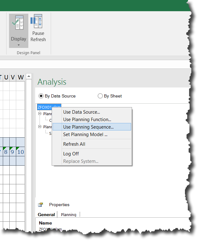
Enter the planning sequence ID = ZSEQ01, search for it and add it to the workbook.

Notice that although the technical name of the sequence is ZSEQ01 the workbook adds an ALIAS = PS_1. You can edit the ALIAS name and make it workbook friendly but we will leave it like that for now.

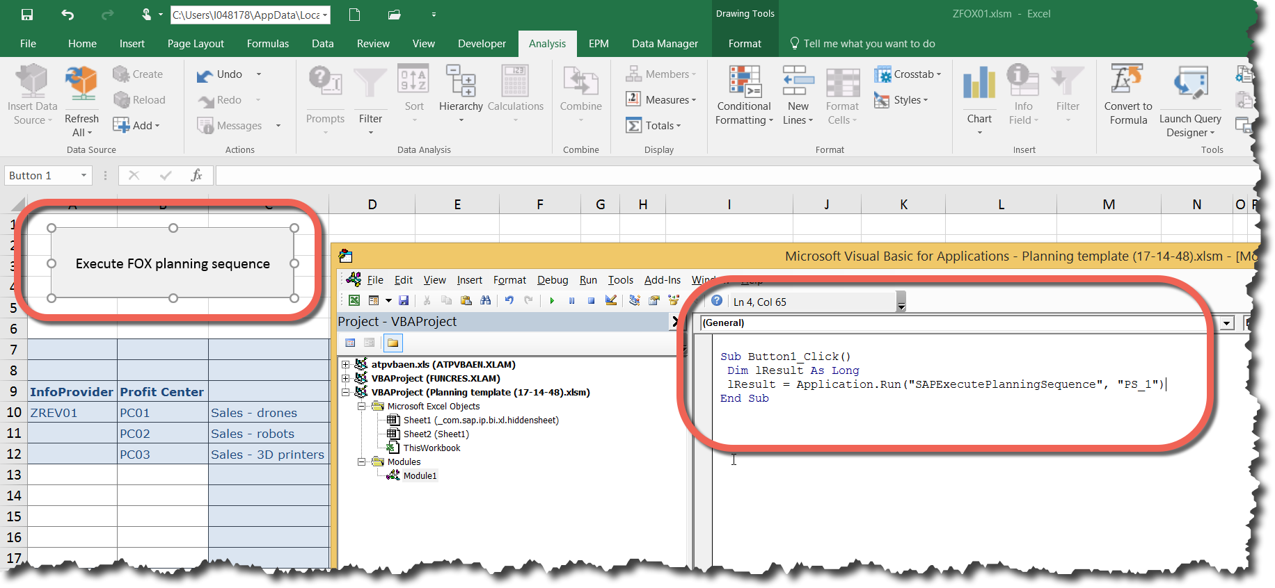
Now from the DEVELOPER ribbon use the TOOLBOX INSERT button to select a BUTTON from the FORM CONTROL and add it to your worksheet in cell A1.

Add the button to the worksheet, give it some appropriate text and link a new macro to it. Select NEW MACRO for the button and add the two lines of code "Dim lResult As Long" and "lResult = Application.Run("SAPExecutePlanningSequence", "PS_1") as shown in the screen shot. Use the ALIAS and NOT the planning sequence ID. Save. Return to the worksheet.
Step 6 - Execute the code
The moment of truth has arrived!! Press the button.
Before:

The destination column is a floating point number key figure so it reflects the decimal precision and we are expecting the sequence to execute and perform our calculations and copy and write new values to periods 1, 2 and 3.

After:

After the button is pressed we see the following results as per our code:
1. {Number, Period 1} = {Quantity, Period 1}
2. {Number, Period 2} = {Quantity, Period 1} * 2
3. {Number, Period 3} = {Number, Period 1} + {Number, Period 2}

1 Comment
You must be a registered user to add a comment. If you've already registered, sign in. Otherwise, register and sign in.
Labels in this area
Related Content
- Manage dates-driven planning processes with SAP Analytics Cloud in Financial Management Blogs by SAP
- Payment Batch Configurations SAP BCM - S4HANA in Financial Management Blogs by Members
- SAP ECC Conversion to S/4HANA - Focus in CO-PA Costing-Based to Margin Analysis in Financial Management Blogs by SAP
- TRM - Error Document type TRO is not defined in Financial Management Q&A
- What’s New in S/4HANA 2023 for IS-Oil and Gas in Financial Management Blogs by Members
Top kudoed authors
| User | Count |
|---|---|
| 5 | |
| 3 | |
| 2 | |
| 1 | |
| 1 | |
| 1 | |
| 1 | |
| 1 | |
| 1 | |
| 1 |