
- SAP Community
- Products and Technology
- Technology
- Technology Blogs by SAP
- Data Wrangling
Technology Blogs by SAP
Learn how to extend and personalize SAP applications. Follow the SAP technology blog for insights into SAP BTP, ABAP, SAP Analytics Cloud, SAP HANA, and more.
Turn on suggestions
Auto-suggest helps you quickly narrow down your search results by suggesting possible matches as you type.
Showing results for
former_member35
Explorer
Options
- Subscribe to RSS Feed
- Mark as New
- Mark as Read
- Bookmark
- Subscribe
- Printer Friendly Page
- Report Inappropriate Content
04-12-2018
10:30 AM
Preparing data can be a tedious and time consuming business, and something that some analysts don’t spend sufficient time on. One of the common initial approaches is to examine the distribution of the data and detect outliers. Depending on the type of algorithm you’re going to use, the data distributions can affect the accuracy of your model, so if you’re using R or SAP HANA Predictive Analytics Library (PAL) you must consider the “skewness” of your data and adjust accordingly. In today’s blog, I’ll review just what I mean by skewed data and why transforming it is so critical.
In probability theory and statistics, “skewness” is a measure of the asymmetry of the data distribution about its mean—it basically measures how “balanced” the distribution is.
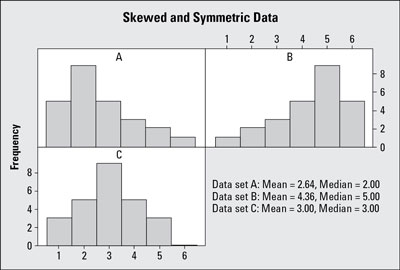
Histogram A shows a “right-skewed” distribution that has a long right tail. Right-skewed distributions are also called “positive-skewed” distributions. That’s because there is a long tail in the positive direction. The mean is also to the right of the peak. The few larger values bring the mean upwards but don’t really affect the median. So, when data are skewed right, the mean is larger than the median.
Common examples for right skewness include:
Right-skew is observed more often than left-skew, especially with monetary type variables. The right-skew results in the mean value not being representative of a typical value for the variable, and this is the reason that the median rather than the mean is often used.
Histogram B shows a “left-skewed” distribution that has a long left tail. Left-skewed distributions are also called “negatively-skewed” distributions. That’s because there is a long tail in the negative direction. The mean is also to the left of the peak. The few smaller values bring the mean down, and again the median is minimally affected (if at all). When data are skewed left, the mean is smaller than the median.
There are fewer real world examples of left skewness:
Histogram C in the figure shows an example of symmetric data. With symmetric data, the mean and median are close together. This can be represented by a normal distribution (the “bell shaped” curve) which is balanced and has no skew.
The detection of skewed data can be an extremely important consideration depending on the type of algorithm you choose to use. One of the assumptions that some algorithms make regards the distribution of data having a normal distribution, where the data is symmetric about the mean.
For example, linear regression, k-nearest neighbour and K-means algorithms are sensitive to the skewness of the data. These algorithms assume that variables have a normal distribution and significant deviations from this assumption can affect the model accuracy and model interpretation. For example, when data has a positive-skew, the positive tail of the distribution will produce models with “bias” where the regression coefficients and influence of variables are more sensitive to the tails of the skewed distribution than they would be if the data had a normal distribution.
This can be demonstrated with a simple linear regression. This algorithm fits the best model by computing the square of the errors between the data points and the trend line.

In the diagram above, you see that the error for the x-axis value, with the outlier value equal to 300, is 70 units. Remember the regression model computes the square of the error, so this value has a large influence on the model.
If this skewed value is removed, then the model is totally different, which you can see from the equation of the line (shown in the red ring):

To minimize the square of the errors, the regression model tries to keep the line closer to the data point at the right extreme of the plot, and this gives this data point a disproportionate influence on the slope of the line.
Apart from linear regression, clustering methods such as K-Means and Kohonen use the Euclidean distance that computes the sum of the squares between the data points, and therefore the skew has the same disproportionate effect. Other algorithms, such as decision trees, are unaffected by skew.
This is why data scientists spend a huge amount of time transforming the data, so that the skewed distribution becomes more like a normal distribution before they build a model. Ideally, for most modelling algorithms, the desired outcome of skew correction is a new version of the variable that is normally distributed.
However, trying to interpret the model with these transformations and explaining to a customer why the log of a variable is preferable to the actual value can be tricky.
Therefore, the detection of skew and the transformation of skewed data is critical if you use some common algorithms such as linear regression, k-nearest neighbour, and K-Means.
So, if you use SAP Predictive Analytics expert mode, SAP HANA PAL, or R, then don’t forget to analyse the distributions and transform your data where necessary. It’s also worth remembering that you don’t need to create transformations if you use SAP Predictive Analytics automated mode. I’ll cover this in more detail in a later blog.
In probability theory and statistics, “skewness” is a measure of the asymmetry of the data distribution about its mean—it basically measures how “balanced” the distribution is.
Right-Skewed Data
Histogram A shows a “right-skewed” distribution that has a long right tail. Right-skewed distributions are also called “positive-skewed” distributions. That’s because there is a long tail in the positive direction. The mean is also to the right of the peak. The few larger values bring the mean upwards but don’t really affect the median. So, when data are skewed right, the mean is larger than the median.
Common examples for right skewness include:
- People's incomes
- Mileage on used cars for sale
- House prices
- Number of accident claims by an insurance customer
- Number of children in a family
Right-skew is observed more often than left-skew, especially with monetary type variables. The right-skew results in the mean value not being representative of a typical value for the variable, and this is the reason that the median rather than the mean is often used.
Left-Skewed Data
Histogram B shows a “left-skewed” distribution that has a long left tail. Left-skewed distributions are also called “negatively-skewed” distributions. That’s because there is a long tail in the negative direction. The mean is also to the left of the peak. The few smaller values bring the mean down, and again the median is minimally affected (if at all). When data are skewed left, the mean is smaller than the median.
There are fewer real world examples of left skewness:
- One is the amount of time students use to take an exam (some students leave early, more of them stay later, and many stay until the end)
- Age at death is negatively skewed in developed countries
Symmetric Data
Histogram C in the figure shows an example of symmetric data. With symmetric data, the mean and median are close together. This can be represented by a normal distribution (the “bell shaped” curve) which is balanced and has no skew.
The detection of skewed data can be an extremely important consideration depending on the type of algorithm you choose to use. One of the assumptions that some algorithms make regards the distribution of data having a normal distribution, where the data is symmetric about the mean.
For example, linear regression, k-nearest neighbour and K-means algorithms are sensitive to the skewness of the data. These algorithms assume that variables have a normal distribution and significant deviations from this assumption can affect the model accuracy and model interpretation. For example, when data has a positive-skew, the positive tail of the distribution will produce models with “bias” where the regression coefficients and influence of variables are more sensitive to the tails of the skewed distribution than they would be if the data had a normal distribution.
This can be demonstrated with a simple linear regression. This algorithm fits the best model by computing the square of the errors between the data points and the trend line.
In the diagram above, you see that the error for the x-axis value, with the outlier value equal to 300, is 70 units. Remember the regression model computes the square of the error, so this value has a large influence on the model.
If this skewed value is removed, then the model is totally different, which you can see from the equation of the line (shown in the red ring):
To minimize the square of the errors, the regression model tries to keep the line closer to the data point at the right extreme of the plot, and this gives this data point a disproportionate influence on the slope of the line.
Apart from linear regression, clustering methods such as K-Means and Kohonen use the Euclidean distance that computes the sum of the squares between the data points, and therefore the skew has the same disproportionate effect. Other algorithms, such as decision trees, are unaffected by skew.
Transforming a Skewed Distribution before Building a Model
This is why data scientists spend a huge amount of time transforming the data, so that the skewed distribution becomes more like a normal distribution before they build a model. Ideally, for most modelling algorithms, the desired outcome of skew correction is a new version of the variable that is normally distributed.
- For positive skew, common corrections are the log transform, multiplicative inverse and square root. These operate by reducing the larger values more and reducing the smaller values less.
- For negative skew, a power transform (like the square, cube, or a higher power) is often used.
However, trying to interpret the model with these transformations and explaining to a customer why the log of a variable is preferable to the actual value can be tricky.
Therefore, the detection of skew and the transformation of skewed data is critical if you use some common algorithms such as linear regression, k-nearest neighbour, and K-Means.
So, if you use SAP Predictive Analytics expert mode, SAP HANA PAL, or R, then don’t forget to analyse the distributions and transform your data where necessary. It’s also worth remembering that you don’t need to create transformations if you use SAP Predictive Analytics automated mode. I’ll cover this in more detail in a later blog.
Learn More
- If you found this post helpful, check out my openSAP course, Getting Started with Data Science.
- Read the other blog posts in our Machine Learning Thursdays series.
- SAP Managed Tags:
- Data and Analytics,
- SAP Predictive Analytics
Labels:
You must be a registered user to add a comment. If you've already registered, sign in. Otherwise, register and sign in.
Labels in this area
-
ABAP CDS Views - CDC (Change Data Capture)
2 -
AI
1 -
Analyze Workload Data
1 -
BTP
1 -
Business and IT Integration
2 -
Business application stu
1 -
Business Technology Platform
1 -
Business Trends
1,661 -
Business Trends
88 -
CAP
1 -
cf
1 -
Cloud Foundry
1 -
Confluent
1 -
Customer COE Basics and Fundamentals
1 -
Customer COE Latest and Greatest
3 -
Customer Data Browser app
1 -
Data Analysis Tool
1 -
data migration
1 -
data transfer
1 -
Datasphere
2 -
Event Information
1,400 -
Event Information
65 -
Expert
1 -
Expert Insights
178 -
Expert Insights
280 -
General
1 -
Google cloud
1 -
Google Next'24
1 -
Kafka
1 -
Life at SAP
784 -
Life at SAP
11 -
Migrate your Data App
1 -
MTA
1 -
Network Performance Analysis
1 -
NodeJS
1 -
PDF
1 -
POC
1 -
Product Updates
4,577 -
Product Updates
330 -
Replication Flow
1 -
RisewithSAP
1 -
SAP BTP
1 -
SAP BTP Cloud Foundry
1 -
SAP Cloud ALM
1 -
SAP Cloud Application Programming Model
1 -
SAP Datasphere
2 -
SAP S4HANA Cloud
1 -
SAP S4HANA Migration Cockpit
1 -
Technology Updates
6,886 -
Technology Updates
408 -
Workload Fluctuations
1
Related Content
- Iterating through JSONModel with multiple nested arrays in Technology Q&A
- Enabling Support for Existing CAP Projects in SAP Build Code in Technology Blogs by Members
- Vendor Invoice Screen 'Payment' tab screen field 'DTWS1' update in Technology Q&A
- I have data like Date, Net, Gross. I want to derive values by Week Range text as dimension in Technology Q&A
- ABAP Cloud Developer Trial 2022 Available Now in Technology Blogs by SAP
Top kudoed authors
| User | Count |
|---|---|
| 13 | |
| 10 | |
| 10 | |
| 9 | |
| 8 | |
| 7 | |
| 6 | |
| 5 | |
| 5 | |
| 5 |