In this blog, we’ll discuss Text Mining which is another interesting area explored by Data Scientist these days. Next Blogs would be Text Mining Functions [
https://blogs.sap.com/2018/02/18/sap-hana-text-mining-functions-part1/], [
https://blogs.sap.com/2018/02/18/sap-hana-text-mining-functions-part2/].
In simple terms, Mining and Analysing text data is used to
- Discover interesting patterns as a part of pattern finding
- Extract useful knowledge as part of knowledge discovery
- Support decision making in businesses
Text Mining provides functionality to compare documents by examining the terms used within documents. Text mining benefits information determined by text analysis which is pre-requisite for text mining. As mentioned in earlier blog Text analysis does linguistic analysis and extracts information embedded within a document while Text mining makes semantic determinations about overall content of a document relative to other documents. Refer to blog on SAP HANA Text Analysis[
https://blogs.sap.com/2018/02/01/sap-hana-text-analysis-3/].
Figure 1 shows an example of Text mining providing key terms and document categorization.

Figure 1: Text Mining – Key Terms and Document Categorization
*****************************************************************************
Text Mining Index
Text Mining maintains a data structure called as Term Document Matrix or Text Mining Index. Terms are relevant words, phrases and entities occurring in document. Term Document matrix is prepared by analyzing set of documents where each column is a document, each word is one of the terms and each cell or element represent term weight as seen in Figure 2.
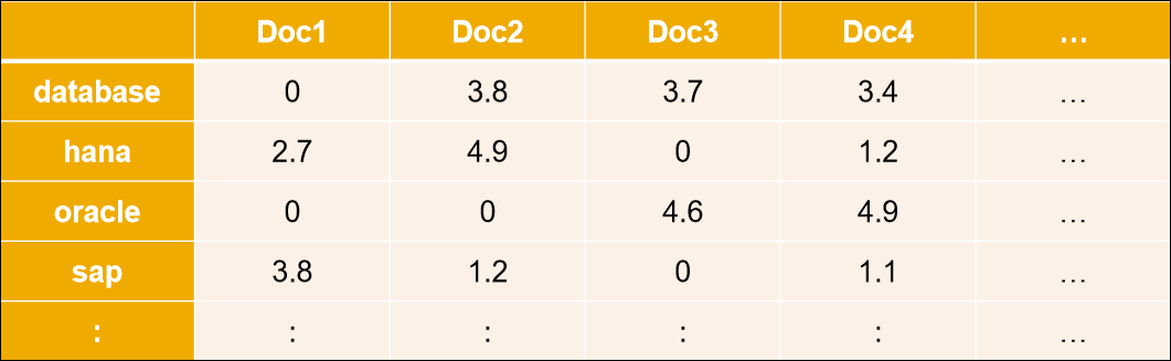
Figure 2: Term Document Matrix
Text Mining assigns a weight to each term in a document to represent its importance. Find below the few Term Weights related to Text Mining.
- Term Frequency
- Document Frequency
- Inverse Document Frequency
- Default Term Weight
Term Frequency(TF) and Normalized Term Frequency(NTF): Number of occurrences of term in document.
Explaining the Term and Normalized Term Frequency using the below example:
Document1: Never Stop Learning in life.
Document2: Life never stop teaching
Document3: The game of life is a game of everlasting learning
Figure 3 shows the Term Frequency in three documents.

Figure 3: Term Frequency
Its recommended to
normalize the document based on size as document size might be large. Normalization is to divide the term frequency by the total number of terms. Figure 4 shows the Normalized Term Frequency in three documents.

Figure 4: Normalized Term Frequency
Document Frequency(DF): Number of documents in which term occurs. Figure 5 shows the Document Frequency for each term.

Figure 5: Document Frequency
Inverse document Frequency(IDF): Reciprocal of DF divided by total number of documents.
IDF(term1) = 1 + log
e(Total Number Of Documents / Number Of Documents with term term1 in it)
There are 3 documents in all = Document1, Document2, Document3
The term game appears in Document3
IDF(game) = 1 + log
e(3 / 1) = 1 + 1.098726209 = 2.098726209
Figure 6 shows the Inverse Document Frequency for each term.

Figure 6: Inverse Document Frequency
Default Term Weight(TF-IDF): TF-IDF compensates the noise words that appear in all documents. Formula: TF * IDF.
For each term in the query multiply its term frequency/normalized term frequency with its IDF on each document. In Document1 for the term life the normalized term frequency is 0.2 and its IDF is 1. Multiplying them together we get 0.2 (0.2 * 1). Figure 7 shows Default Term Weight.

Figure 7: Default Term Weight
Syntax of creating Text Mining Index
CREATE FULLTEXT INDEX [INDEX NAME] ON [SCHEMA].[TABLE]([COLUMN]) FAST PREPROCESS OFF TEXT MINING ON;
MERGE DELTA OF [SCHEMA].[TABLE];
Requirements:
- Column table with character or binary content (same requirement as for text analysis)
- FAST PREPROCESS OFF (required for text analysis and text mining)
- Delta changes must be merged to main table storage first using MERGE DELTA SQL statement
Figure 8 shows the relation between Database table and Full Text Index.

Figure 8: Relation between Database table and Text Mining Index
For details on Full Text Indexing refer to blog [
https://blogs.sap.com/2018/02/15/sap-hana-full-text-index/].
************************************************************************************
“Bag of Words” Model for Comparison
Text Mining compares documents using “Bag of Words” Model. The “Bag-of-words” model is used to represent text in bag(multiset) of words or list of vectors, disregarding grammar and order of words but keeping multiplicity of words.
The following example models a text document using bag-of-words.
Text document contains
Bob likes to play soccer.
Bob dislikes Football.
Based on text document, a list is constructed as follows:
“Bob”
“Likes”
“To”
“Play”
“Soccer”
“Dislikes”
“Football”
N-dimensional vector space model for checking Similarity
Text mining compares the similarity of two documents by comparing the relative weights of the terms they contain. The comparison is done using an N-dimensional vector space model. Similarity of two documents is related to how much their vectors point in same direction. Text mining now supports below listed standard similarity measures: COSINE, JACCARD, DICE and OVERLAP.
Cosine Similarity: Most commonly used is cosine similarity. To understand the similarity measures, we’ll start with the explanation of vector and Euclidean dot product. From each document, a vector is derived. The set of documents is viewed as a set of vectors in a vector space. Each term will have its own axis.
Vector has a magnitude and direction as shown in Figure 9a.

Figure 9a Vector
Euclidean Dot Product of two vectors shown in Figure 9b can be calculated as
a · b = |a| × |b| × cos(θ)
Where
|a| is the magnitude (length) of vector a
|b| is the magnitude (length) of vector b
θ is the angle between a and b

Figure 9b Euclidean Dot Product
When two documents are similar, they will be relatively close to each other in vector space which means they’ll point in same direction from the origin forming a small angle. Whereas if the two documents are dissimilar, their points will be distant, and likely to point in different directions from the origin, forming a wide angle. The cosine of the angle leads to a similarity value.
Cosine similarity values range from -1 to 1
- Cosine similarity of vectors at 0° is 1 which indicates exactly same orientation
- Cosine similarity of vectors at 90° is 0 which indicates orthogonality (decorrelation)
- Cosine similarity of vectors at 180° is “−1” means exactly diametrically opposite while in-between values indicates intermediate similarity or dissimilarity.
Formula for cosine similarity:
Cosine Similarity (d1, d2) = Dot product (d1, d2) / ||d1|| * ||d2||
Dot product (d1, d2) = d1[0] * d2[0] + d1[1] * d2[1] * … * d1[n] * d2[n]
||d1|| = square root(d1[0]
2 + d1[1]
2 + ... + d1[n]
2)
||d2|| = square root(d2[0]
2 + d2[1]
2 + ... + d2[n]
2)
To summarize, Text Mining provides functionality to compare documents by examining the terms used within documents.
